By Lacy Hunt, PhD, and Van Hoisington, Hoisington Investment Management
Nearly nine years into the current economic expansion Federal Reserve policy actions appear to be benign, as even after six increases, the federal funds rate remains less than 2%. Changes in the reserve, monetary and credit aggregates, which have always been the most important Fed levers both theoretically and empirically, indicate however that central bank policy has turned highly restrictive. These conditions put the economy’s growth at risk over the short run, while sizable increases in federal debt will serve to diminish, not enhance, economic growth over the long run.
Interest Rates
Interest rates are not predictable over the short run but are controlled by fundamental forces on a long-term basis. Milton Friedman (1912- 2006) developed the most complete and internally consistent interest rate model to date, which is an extension of the Fisher equation. Friedman’s model reaches two conclusions: (1) although monetary decelerations may lead to transitory increases in interest rates over the short run, they ultimately lead to lower rates; and (2) monetary accelerations result in higher rates. This reasoning is based on what Friedman termed “liquidity, income and price effects”. When the Fed reduces the reserve, monetary and credit aggregates (or what Friedman called monetary deceleration), initially short-term rates are forced upward through the “liquidity (or initial) effect”. As the Fed further tightens monetary conditions, an offsetting “income effect” follows. These restraining actions moderate growth in the economy, and the rise in interest rates continues but at a slower pace. Thus, in Friedman’s terms, the income effect begins to offset the liquidity effect. When the Fed sustains the tightening process long enough, the inflation rate will decrease as incomes fall and ultimately result in lower rates. This is the “price” or “Fisher effect” from the Fisher equation. Observationally, the highly inflation-sensitive long-term yields reflect the changing economic landscape faster than short-term rates, thus the yield curve flattens, serving to strengthen the Fed’s restraint on the reserve, monetary and credit aggregates.
Empirical studies by Friedman and others indicate this process is lengthy, often playing out over several years. This process appears to be well underway. More than two years have elapsed since the Fed initiated the liquidity effect, and restraint is evident in all of the aggregates as well as in the shape of the yield curve, which has attened significantly.
Friedman's logic for monetary accelerations leading to higher interest rates is the opposite of monetary decelerations. When the Fed accelerates growth in the reserve, monetary and credit aggregates, the liquidity effect is initiated. Short term rates drop rapidly relative to long term rates and the yield curve dramatically steepens. If the Fed continues to further loosen monetary conditions, a reversing income and price effect can, but does not always, occur. Friedman assumed the velocity of money was largely stable. Subsequent empirical evidence, however, suggests that this is not the case.
Three important concepts arise from these patterns. First, when the Fed moves in one direction, they ultimately lay the groundwork for reversal. Second, considerable time (generally two or more years) passes before the liquidity effect has any economic impact. Third, these lags grow longer when the Fed tries to overcome a recession, especially in highly leveraged economies like 1929 and 2008.
The Fed's Ability to Act
The fact that there is such a long lag between policy change and economic impact is critical in analyzing the circumstances today. For instance, suppose the Fed is able to identify the next recession on day one. Also, suppose that on the first day of the recession the Fed drops the federal funds rate to zero. Due to the economy’s extreme over-indebtedness, along with long monetary policy lags, a minimum of one and half years could elapse before even a slight economic recovery is experienced. But, recovering from the next recession, the lag could be much longer since interest rates are so close to the zero bound and indebtedness continues to rise to record levels. Both will interfere with the potency of the liquidity effect. Thus, despite a rapid Fed response, a long recession could ensue.
Monetary Decelerations and Recessions – the Historical Record
Since the early 1900s, money supply (M2) decelerated prior to 17 of the 21 recessions (Chart 1). This strong correlation is remarkable given the complexity of the economy and shifting initial conditions. The lead times between the peaks in M2 growth and the start of the next recession are variable, with many centered around two years; however, some are shorter and others are as long as three years. The variability in lag times is far from surprising due to widely varying initial conditions: degree of leverage, demographics, global conditions and a host of other variables. When an economic model does not fully explain all of the historical experiences, the best approach is to study the cases that appear to contradict the normal pattern. The four deviating instances are labeled A, B, C, and D (Chart 1).
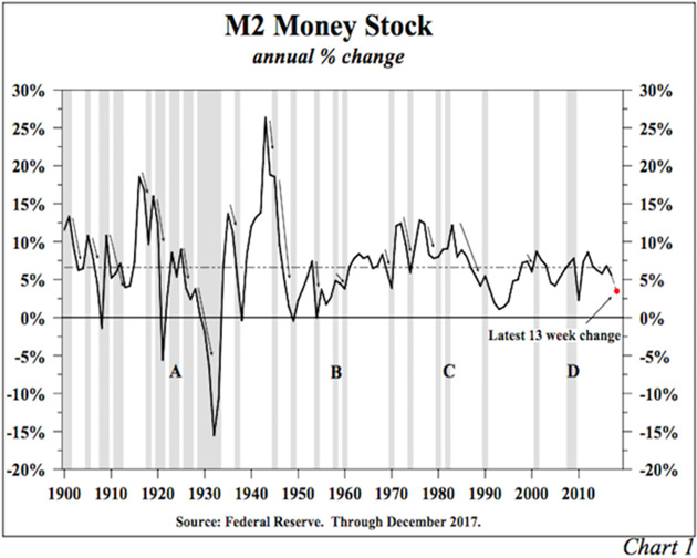
At point A, the money supply did not decelerate prior to the 1923 recession, but money velocity fell as the economy became increasingly leveraged. (This is important because the equation of exchange posits that money times velocity equals nominal GDP (M*V = NGDP).) The treasury yield curve significantly flattened and so did the corporate yield curve, which at the time was a more important indicator.
At point B, M2 did not decelerate prior to the 1958 recession. In this case the rate of growth in the monetary base sharply decelerated along with bank credit. Additionally, the treasury yield curve inverted.
At point C, if the 1980 and 1981-82 recessions are counted as one recession, as many prominent economists suggest, M2 growth did decelerate sharply prior to the downturn. Moreover, all of the monetary variables denote that severe restraint had been initiated to contain double-digit inflation. In other words, no contradiction existed as monetary policy tightened, and then the economy collapsed.
At point D (or prior to 2008), M2 growth did not decelerate until the economy was already in recession. However, the entire set of other monetary variables was restrictive.
Therefore, in the four instances when M2 growth failed to signal the downturn, M2’s closely aligned partners, on balance, pointed to recession.
Using the Brunner-Meltzer Model to Explain Collapsing Money and Bank Credit Growth Rates
M2 is largely measured from the liability side of bank balance sheets. Bank credit, which includes loans and investments or security holdings, is the aggregate of bank assets. Economists Karl Brunner (1916-1989) and Allan Meltzer (1928- 2017) developed the money supply determination model used in all major macroeconomic texts. This algebraically proven model states that M2 equals the monetary base times the money multiplier (m).
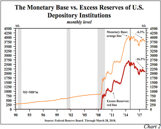
Since late 2015, in large part due to the Fed’s actions of raising the federal funds rate and more recently reducing the Fed balance sheet (quantitative tightening or QT), the monetary base has registered a pronounced decline of 6.3%. Excess reserves of the depository institutions fell by more than 16% over this time. Part of this decline may be attributed to other volatile factors rather than to changes in the Fed’s balance sheet. Taking these factors into account and smoothing out fluctuations in excess reserves, it appears that each increase in the federal funds rate required that excess reserves decrease by approximately $68 billion. This accounts for the approximate $410 billion decline in excess reserves. Due to quantitative tightening, the Fed balance sheet was reduced by $57 billion in the past two quarters. Using excess reserves, rather than the fed funds rate, as a measure of Fed tightening, we conclude the Fed has engaged in the equivalent of closer to seven increases in the federal funds rate rather than the six increases reported. This exercise is to highlight that the Fed policy of reducing its balance sheet is measurably more restrictive than their stated policy tool (fed funds).
At the start of the first quantitative easing (QE1), Fed Chairman Bernanke said the Fed was printing money. Due to the Fed’s balance sheet, the monetary base surged, but M2 did not respond due to the decline of m. (Remember, m is the equal partner to the base.) Some might presume that if m declined during QE, it would rise during QT. But currently the determinants of m – excess reserves, time and savings deposits, currency, and treasury ratios – have worked in tandem to cause m to stabilize. Thus, together, reductions in the base and m have caused the rate of growth in M2 and commercial bank credit (the sum of loans and investments) to slow noticeably.
Until the Federal Reserve Act of 1937 is repealed, m will remain algebraically defined. The Fed can neither print money nor reverse the printing press. The Federal Reserve can raise or lower the monetary base, but no certainty exists that there will be a correspondingly desired change in the money supply or bank credit, unless m cooperates. Conclusively, the Fed’s balance sheet and m are of equal importance. The widely held presumption that the Fed policy of QE would work, reflects that the Brunner-Meltzer model was not properly understood.
In the first quarter of 2018, M2 growth decelerated to just above a 2% annual rate. Year- over-year M2 growth slowed to just 3.9% versus the 6.6% long-term average growth. Additionally, bank credit growth declined 0.6% at an annual rate. Loans continued to inch upward but only because the banks’ securities portfolios fell. Loan volume does not typically fall until an economy is in a recession because firms borrow to finance an unintended rise in inventories.
The proposition that the federal funds rate is the major policy tool to control economic activity is greatly flawed. As the past ten years have proven, the Fed faces a difficult task of working with both price (interest rate) and quantity (money supply) to influence economic activity. Present circumstances reveal extraordinarily low money growth, tighter bank liquidity (Chart 2), and the inability of several sectors to borrow due to higher rates. The historical record of these Fed actions points toward a continuing pattern of economic deterioration. While the brunt of monetary policy will impact economic growth increasingly over the next two years, the longer run view of economic conditions will be shaped by the exploding level of government debt.
The Debt End Game – The Law of Diminishing Returns
Federal debt continues to rise at an accelerating pace, a trend reinforced by the bipartisan budget enacted March 23rd of this year and the tax cut and reform legislation that went into effect January 1st of this year. These changes occur at a time when many expenditure items have been moved off-budget, causing a wider gap between the issuance of debt and the reported deficit (note: in the last ten scal years, the cumulative budget deficit has been $8.5 trillion while government debt has increased by $11.3 trillion). Additionally, an aging population is set to greatly boost federal debt over the next 15 years. Gross federal debt was 105.4% at year-end 2017, but it could reach 120% before the end of the next decade.
The economic impact of this explosion in debt has been analyzed through a plethora of academic articles. The most germane might be the Checherita and Rother 2010 study which shows that excessive indebtedness is deleterious for economic growth in a non-linear fashion. That is, the higher the level of debt the greater the restraint on economic growth.
While many believe that surging debt will boost economic growth, the law of diminishing returns indicates that extreme indebtedness will impede economic growth and ultimately result in economic decline. Diminishing returns is about economic growth and thus highly important in economics since the standard of living cannot be raised without increasing output. The application of diminishing returns means a disproportionate growth in debt will produce similar results for all countries in extreme debt, regardless of their idiosyncratic conditions. Thus, no matter how U.S., Japanese, Chinese, European or emerging market debt is financed or owned, and regardless of the economic system, the path is stagnation and then decline. Even central bank funding of debt will not negate diminishing returns.
The law of diminishing returns rests upon the production function that states physical output on either a micro or macro scale is a function of the inputs. These inputs – labor, capital and natural resources – are called the factors of production. When a factor of production input (for instance, debt capital) goes up, output rises at an increasing rate and marginal physical product (MPP) also increases. However, as that factor disproportionally continues to increase, MPP experiences slower gains and diminishing returns occur, followed by flat returns. As debt continues to increase, real GDP starts to fall. At this point, debt has reached the point of negative returns, resulting in the end game of extreme indebtedness. Faltering output will free up substantial credit in more than sufficient volume to overwhelm the impact of the ever increasing supply of new debt. Although the business and financial cycles will continue to operate, low interest rates will prevail as debt is used in ever increasing amounts to boost economic output.
While labor, natural resources and equity capital theoretically could increase proportionately with debt capital, these levers are not easily changed and their trends are not positive. Poor demographics in Europe, Japan, the U.S. and China suggest labor will not be a major positive for almost two more decades, even under the most optimistic of scenarios. Equity capital is moving in the wrong direction due to low net U.S. savings along with corporate preferences. Technology will change, but the more deleterious impact may fall on labor and natural resources. Thus, overuse of debt capital is the path of least resistance.
The law of diminishing returns holds important implications for both recent and future fiscal policy actions that have increased, and will continue to increase, federal debt. Suppose that during the next recession the economic solution is assumed to be an even more massive rise in debt than the $3.5 trillion explosion that occurred during and after the recession of 2008-09. This policy will result in even smaller economic gains than in the current expansion. If debt increases are doubled, tripled, or even quadrupled, the law of diminishing returns indicates economic growth will become even more frail.
Mounting Evidence
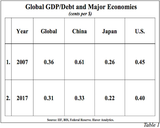
The law of diminishing returns is already evident in all major economies as well as on a global scale (Table 1). Global GDP generated per dollar of total global public and private debt dropped from 36 cents in 2007 to just 31 cents in 2017. Diminishing returns is even more apparent in the case of China’s public and private debt, largely internally owned. In terms of each dollar of debt, China generated 61 cents of GDP growth in 2007 and only 33 cents last year. In other words, in the past ten years the efficiency of China’s debt fell 45%. Thus, even in a command and control economy, the law of diminishing returns prevails. The most advanced sign of diminishing returns is in Japan, the most heavily indebted major country, where a dollar of debt in the last year produced only 22 cents of GDP growth. This economic principle applies equally to businesses.
All economies rely heavily on the business sector to lead the growth process. Yet, a sharp decline in GDP per dollar of business debt occurred in the U.S. during the past nine years, reinforcing the underlying trend since the early 1950s. In 1952, $3.42 of GDP was generated for every dollar of business debt, compared with only $1.39 in 2017. In the corporate sector, where capital as well as technology is most readily available, GDP generated per dollar of debt fell from $4.50 in 1952 to $2.50 in 2007 to $2.21 last year. The dismal trend in productivity confirms this conclusion. The percent change for productivity in the last five years (2017-2012) was equal to the lowest of all five-year spans since 1952. It was also less than half the average growth over that period.
Conclusion
Important to the long-term investor is the pernicious impact of exploding debt levels. This condition will slow economic growth, and the resulting poor economic conditions will lead to lower inflation and thereby lower long-term interest rates. This suggests that high quality yields may be difficult to obtain within the next decade. In the shorter run, in accordance with Friedman’s established theory, the current monetary deceleration, or restrictive monetary policy, will bring about lower long-term interest rates.
Van R. Hoisington
Lacy H. Hunt, Ph.D.


