Smart Beta Returns (Hint: History Is Worse than Useless)

by Rob Arnott Noah Beck Vitali Kalesnik, Research Affiliates

Key Points

• Using past performance to forecast future performance is likely to disappoint. We find that a factor’s most recent five-year performance is negatively correlated with its subsequent five-year performance.
• By significantly extending the period of past performance used to forecast future performance, we can improve predictive ability, but the forecasts are still negatively correlated with subsequent performance: the forecast is still essentially useless!
• Using relative valuations, we forecast the five-year expected alphas for a broad universe of smart beta strategies as a tool for managing expectations about current portfolios and constructing new portfolios positioned for future outperformance. These forecasts will be updated regularly and available on our website.

In a series of articles we published in 2016,1 we show that relative valuations predict subsequent returns for both factors and smart beta strategies in exactly the same way price matters in stock selection and asset allocation. To many, one surprising revelation in that series is that a number of “smart beta” strategies are expensive today relative to their historical valuations. The fact they are expensive has two uncomfortable implications. The first is that the past success of a smart beta strategy—often only a simulated past performance—is partly a consequence of “revaluation alpha” arising because many of these strategies enjoy a tailwind as they become more expensive. We, as investors, extrapolate that part of the historical alpha at our peril. The second implication is that any mean reversion toward the smart beta strategy’s historical normal relative valuation could transform lofty historical alpha into negative future alpha. As with asset allocation and stock selection, relative valuations can predict the long-term future returns of strategies and factors—not precisely, nor with any meaningful short-term timing efficacy, but well enough to add material value. These findings are robust to variations in valuation metrics, geographies, and time periods used for estimation.

Two assumptions widely supported in the finance literature form the basis for how most investors forecast factor alpha and smart beta strategy alpha. We believe both, although strongly entrenched in investors’ thinking, are wrong. The two assumptions we take issue with are that past performance of factor tilts and smart beta strategies is the best estimate of their future performance, and that factors and smart beta strategies have constant risk premia (value-add) over time.

Common sense tells us that current yield begets future return. Nowhere is this more intuitive than in the bond market. Investors fully understand that the average 30-year past return of long bonds, currently north of 7%, tells us nothing about the future return of long bonds. The current yield, around 3%, is far more predictive. In the equity market, at least since the 1980s, we know that the cyclically adjusted price-to-earnings (CAPE) ratio, as demonstrated by Robert Shiller, and the dividend yield are both good predictors of long-term subsequent returns.

If relative valuation, and the implication it has for mean reversion, is useful for stock selection and for asset allocation, why would it not matter in choosing factor tilts and equity strategies? The widespread promotion by the quant community of products based on past performance—often backtests and simulations—has contributed, and still does contribute, to investors’ costly bad habit of performance chasing. The innocent-looking assumption of “past is prologue” conveniently encourages investors and asset managers to pick strategies with high past performance and to presume the past alpha will persist in the future.

In our 2016 smart beta series we offer evidence that relative valuations are important in the world of factors and smart beta strategies. We show that variations in valuation levels predict subsequent returns and that this relationship is robust across geographies, strategies, forecast periods, and our choice of valuation metrics. Our research tells us that investors who (too often) select strategies based on wonderful past performance are likely to have disappointing performance going forward. For many, mean reversion toward historical valuation norms dashes their hopes of achieving the returns of the recent past.

These conclusions are, of course, just qualitative. To make them practical, we need to quantify the effects we observe. In this article we do precisely that. We measure the richness of selected factors based on their relative valuations versus their respective historical norms and calculate their implied alphas. We also call attention to the real-world “haircuts” on the implied alphas—implementation shortfall, trading costs, and manager fees—which don’t show up in paper portfolios and simulations.

Why Valuations Matter

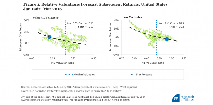
We can easily see the link between valuation and subsequent performance on a scatterplot created using these two variables. The two scatterplots in Figure 1 are from Arnott, Beck, and Kalesnik (2016a) and are examples of the historical distributions of valuation ratios and subsequent five-year returns for a long–short factor, the classic Fama–French definition of value, and for a smart beta strategy (the low volatility index), as of March 31, 2016. In June 2016, we identified the former as the cheapest factor, relative to its history, and the latter as the most expensive strategy, relative to its history.

The value factor consists of a long value portfolio and a short growth portfolio. We measure performance and relative valuation by comparing the value portfolio relative to the growth portfolio. For the low-volatility index we measure performance and relative valuation by comparing the low-volatility portfolio with the cap-weighted stock market. The dotted line shows the average relationship between valuations and subsequent five-year performance. Both scatterplots show negative slope: richer valuations generally imply lower subsequent returns, while cheaper valuations imply higher subsequent returns. We use the same method for other factors and smart beta strategies. For most strategies and factors across multiple geographic regions the relationship is both statistically and economically significant.

Comparing Alpha-Forecasting Models

Many investors expect the alpha of a strategy to be its historical alpha, so much so that this assumption itself is an example of an alpha-forecasting model. One of the cornerstones of any investment process is an estimate of forward-looking return. We argue that a good alpha-forecasting model, whether for a strategy or a factor tilt, should have three key attributes::

1. Forecasts should correlate with subsequent alphas.
2. Forecasts should be paired with a measure of the likely accuracy of the forecast. A standard statistical way to measure the accuracy of a forecast is mean squared error, a measure of how reality has differed from past forecasts.
3. Forecasts should provide realistic estimates of expected returns.

These criteria provide useful metrics for us to compare different alpha-forecasting models. We select six models for comparison. One model assumes an efficient market: no factors or strategies have any alpha. Two of the models use only past performance and ignore valuations, and four of the models are based on valuation levels relative to historical norms.

Model 0. Zero factor alpha. In an early version of the efficient market hypothesis—the capital asset pricing model, or CAPM—researchers argued that an asset’s return was solely determined by its exposure to the market risk factor. Similarly, Model 0 assumes the risk-adjusted alpha of a factor tilt or smart beta strategy is approximately zero. We measure the mean squared error relative to an expected alpha of zero.

Model 1. Recent past return (most recent five years). This model uses the most recent five-year performance of a factor or strategy to forecast its future return. Because our research tells us that investors who select strategies based on wonderful past performance are likely buying stocks with high valuations, we expect this model will favor the strategies that are currently expensive and have low future expected returns.

Model 2. Long-term historical past return (inception to date). Long-term historical factor returns are perhaps the most widely accepted way to estimate factor premiums (expected returns), both in the literature and in the practitioner community. Doing so requires that we extrapolate historical alpha to make the forecast: what has worked in the past is deemed likely to work in the future. Averaging performance over a very long period of time should theoretically mitigate vulnerability to end-point richness.2 By using multiple decades of history (versus a short five-year span as Model 1 does), we would expect this model to perform relatively well in differentiating well-performing factors from less-well-performing ones.

Model 3. Valuation dependent (overfit to data). This model is a simple and intuitive valuation-dependent model, as illustrated by the log-linear line of best fit in Figure 1.3 At each point in time, we calibrate the model only to the historically observed data available at that time; no look-ahead information is in the model calibration. This model encourages us to buy what’s become cheap (performed badly in the past), rather than chasing what’s become newly expensive (has performed exceptionally well).

Model 4. Valuation dependent (shrunk parameters). A model calibrated using past results may be overfitted, and as a result provide exaggerated forecasts that are either too good or too bad to be true. Parameter shrinkage is a common way to reduce model overfitting to rein in extreme forecasts. (Appendix A provides more information on how we modify the parameters estimated in Model 4 to less extreme values.)

Model 5. Valuation dependent (shrunk parameters with variance reduction). Model 5 further shrinks Model 4 by dividing its output by two. The output of this model is perfectly correlated with the output of Model 4, with the forecast having exactly two times lower variability.

Model 6. Linear model (look-ahead calibration). Model 6 allows look-ahead bias. With our log-linear valuation model we estimate using the full sample. Of course, this model will deliver past “forecasts” that are implausibly good because no one has clairvoyant powers! Nevertheless, it provides a useful benchmark—a model that, by definition, has perfect fit to the data—against which we can compare our other models. How close can we come to this impossible ideal?

For our model comparison we use the same eight factors in the US market as we use in our previously published research. (The description of our factor construction methodology is available in Appendix B.) We use the first 24 years of data (Jan 1967–Dec 1990) in the initial model calibration, encompassing several valuation cycles, and use the remaining data (Jan 1991–Oct 2011) to run the model comparison. These data end in 2011 because we are forecasting subsequent five-year performance; an end date in October allowed us to conduct our model comparison analysis in November and December. We report the comparison results in Table 1. Model 0 and Model 2 are our base cases. We need to beat a static zero-alpha assumption (Model 0) in order to even argue for the use of dynamic models in alpha forecasting. And we need to beat Model 2 to demonstrate the usefulness of a valuation-based forecasting model.

Assuming that future alpha is best estimated by the past five years of performance, Model 1 provides the least accurate forecast of alpha (i.e., based on mean squared error (MSE), it performs the worst of all six models). Further compounding its poor predictive ability, its forecasts are negatively correlated with subsequent factor performance. Focusing on recent performance—the way many investors choose their strategies and managers—is not only inadequate, it leads us in the wrong direction.

Model 2, which uses a much longer period of past performance to forecast future performance, provides a significant improvement in accuracy over Model 1, as reflected by a much smaller MSE. Still, as with Model 1, its forecasts are negatively correlated with subsequent performance, and its forecast accuracy is worse than the zero-factor-alpha Model 0.

The key takeaway in the comparison of Models 1 and 2 is that a very long history of returns, covering at least several decades, may provide a more accurate forecast of a factor’s or smart beta strategy’s return than a short-term history, but the forecast is still essentially useless. Selecting strategies or factors based on past performance, regardless of the length of the sample, will not help investors earn a superior return and is actually more likely to hurt them. The negative correlations of the forecasts of both Models 1 and 2 with subsequent factor returns imply that factors with great past performance are likely overpriced and are likely to perform poorly in the future.4

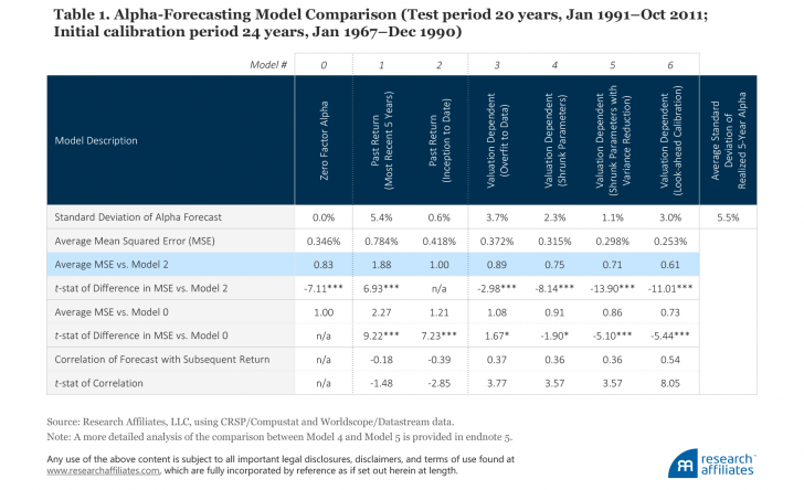
Valuation-dependent Models 3–6 all have positive correlations between their forecasts and subsequent returns, and all beat Model 0 in this regard; the correlation is undefined for Model 0 because its forecasts are always constant. Models 4–6 beat Model 0 in forecast accuracy, with all having a lower MSE than Model 0.

Model 6, which is fit to the full half-century data sample, provides the best forecast of expected return because, of course, it’s hard to beat clairvoyance! The improvement in forecasting error of 39% for Model 6 compared to Model 2 shows how much, at best, a valuation-based model can reduce the error term. Model 3, a linear model that does not use any look-ahead information in its calibration, reduces the error term by 11% compared to Model 2—nice, but not impressive—and its errors are a bit larger than the naïve assumption that all alphas are zero.

Model 4, which does not use look-ahead information in its calibration, reduces the error term by 25% versus Model 2, roughly two-thirds as good as clairvoyance! All four models that forecast using valuations (Models 3–6) are able to substantially improve forecast accuracy compared to Models 1 and 2, which use only past returns.5

Model 4 shrinks parameter estimates away from extreme values, mitigating the risk of overfitting the data. It also provides a more realistic out-of-sample alpha forecast compared with Model 5. We therefore apply it in the next section (while cheerfully acknowledging it could likely be further improved) to investigate what current valuations are telling us about the alpha forecasts for factors and smart beta strategies. Readers who are more interested in the current forecasts of Model 5, which is also a very good model, merely need to cut these forecasts in half.

Factor and Smart Beta Strategy Alpha Forecasts

Using Model 4, we calculate the alpha forecasts over the next five-year horizon for a number of factors and smart beta strategies.6

Factors

We find that almost all popular factors in the US, developed, and emerging markets have shown strong historical returns. This outcome is utterly unsurprising: the road to popularity for a factor or a strategy is high past performance. The only popular factors with negative (but insignificant) past performance are illiquidity and low beta in the developed markets, and size in the emerging markets.

Figure 2, Panel A, plots the historical excess return and historical volatility, and Panel B the five-year expected return and expected volatility, at year-end 2016 for a number of common factors in the US market, constructed as long–short portfolios. We provide the same data for the developed and emerging markets in Appendix C. (The results can also be found in tabular form later in the article in Table 2, Panel A.) The alpha forecasts are plotted against the projected volatilities, which are estimated as an extrapolation of recent past volatility.7

The volatilities of the factor portfolios are a measure of the volatility of a long–short portfolio; in other words, these volatilities measure the volatility of the return difference between the long and the short portfolios. Take, for example, the low beta factor in the United States, which has a volatility second only to the momentum factor. Does this mean that low beta stocks have high volatility? No. The factor portfolio that goes long in low beta stocks and short in high beta stocks carries with it a substantial negative net beta, which contributes to the volatility of the factor.8

The volatility of the low beta factor in this long–short framework therefore suggests that a long-only low beta investor should expect large tracking error with respect to the market, even if the portfolio is much less risky than the market. Momentum also typically leads to high tracking error, while the investment factor leads to low tracking error. Viewing projected alpha and relative risk together gives us an insight into the likely information ratios currently available in these factors.

Factors with negative forecasted alpha. Forecasted alphas for low beta factors are negative in all markets. Having experienced a strong bull market from 2000 through early 2016, and even after a large pullback over the second half of 2016, low beta factors are still quite expensive relative to their historical valuation norms. We hesitate to speculate if this is due to the rising popularity of the factor driving the relative valuation higher or the soaring valuation driving the rising popularity. As anyone in the social sciences knows, correlation is not causation. Either way, the data suggest we should not expect low beta strategies to add much value to investor portfolios until their valuations are more consistent with their past norms.

We also hesitate to dismiss the low beta factor solely because of its relative valuation. Diversification and the quest for return are both important goals. Even at current valuation levels, low volatility can serve an important role in both reducing and diversifying risk. A sensible response is to rely on the low beta factor less than we might have in the past.

Alpha forecasts for the size factor (small cap versus large cap) are negative in all markets. Put another way, the size factor in all regions is expensive relative to its own historical average. In the United States this relationship has flipped from a year ago: the Russell 2000 Index beat the Russell 1000 Index by over 1,000 bps in the second half of 2016. This huge move takes the size factor (in the United States) from somewhat cheap a year ago to neutral now. Size has lower long-term historical performance compared to other factors in most regions, so modest overvaluation (outside the United States) is enough to drive our alpha forecasts negative. Other factors with less attractive projected alphas are illiquidity in the US market and gross profitability in the developed markets, both forecast to have close to zero expected return over the next five years.

Factors with positive forecasted alphas. Value outperformed handily in 2016, but not enough to erase the relative cheapness of the strategy in most markets, especially in the emerging markets. Increasing valuation dispersion around the globe has opened up many great opportunities for the patient value investor, the mirror image—tumbling popularity, tumbling relative valuations, and tumbling historical returns—of the picture painted by low beta.

We look at value two ways. The first, a composite, is one of the factors with the highest projected expected returns across all regions. The composite is constructed using four valuation metrics, each measuring the relative valuation multiples of the long portfolio (value) relative to the short portfolio (growth): Price to book value (P/B), price to five-year average earnings (P/E), price to five-year average sales (P/S), and price to five-year average dividends (P/D).

The second value factor we construct is based on P/B, the classic measure most favored in academe. Unlike the value composite, it has close to zero projected return. The lower forecasted return may be associated with the big gap in profitability observed among companies today versus in the past. A strategy favoring high B/P companies may favor less profitable companies, increasing investor exposure to “value traps”—those companies that look cheap on their way to zero!

After a lousy second half of 2016, momentum has flipped from overpriced to underpriced. Is this because momentum underperformed so drastically that it’s now cheap? No. Its composition changed. A year ago, the FANGs (Facebook, Amazon, Netflix, and Google) had great momentum—the momentum factor was signaling “buy.” Value stocks are handily outpacing growth now, and value has the momentum. It turns out that, although for most factors relative valuation plays out slowly over a number of years, valuation is a pretty good short-term predictor for momentum performance. Across all markets, we expect momentum to deliver respectable future performance slightly above historical norms. The “signal” changes pretty rapidly from year to year (and sometimes even from month to month).

Finally, we are projecting good performance for gross profitability in the US market over the next five years, a switch from last spring. Quality’s disappointing performance in the second half of 2016 sowed the seeds for this turn in relative attractiveness.

Our return forecasts are all before trading costs and fees. In the real world, these anticipated costs should be subtracted from return forecasts to reflect the investor’s true expected return. In the case of momentum, trading costs can dwarf fees.

Smart Beta Strategies

In addition to factors, which are theoretical difficult-to-replicate long–short portfolios, we estimate the expected risk–return characteristics for a selection of the more-popular smart beta strategies. The list of strategies and the description of their methodologies is available in Appendix B. In order to produce forecasts we replicate the strategies using the published methodologies of the underlying indices. Any replication exercise is subject to deviation from the original due to differences in databases, rebalancing dates, interpretations of the written methodologies, omitted details in the methodology description, and so forth; our replication is no exception.9 The results of the replicated exercise, albeit imprecise, should be informative of the underlying strategies.10

The results for the smart beta strategies yield a number of interesting observations, some of which are quite similar to our observations about factors. Like popular factors, all popular strategies in all regions (with the exception of small cap in emerging markets) have positive historical returns. Again, this should not be surprising because these strategies would not be popular without strong historical returns! Note many of the strategies are simulated backtests for most of the historical test span. Accordingly, as with factors, the high historical returns for long-only investment strategies should be adjusted downward for selection bias.11

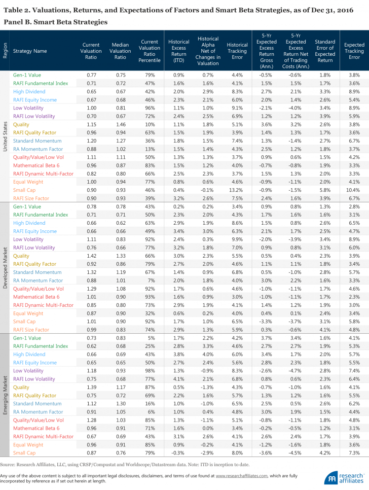
The historical and expected alphas for the smart beta strategies, as well as their respective tracking errors, implied by current US valuation levels are shown in the scatterplots in Figure 3. Appendix D presents the same data for the developed and emerging markets. (The data are also provided in tabular form later in the article in Table 2, Panel B.)

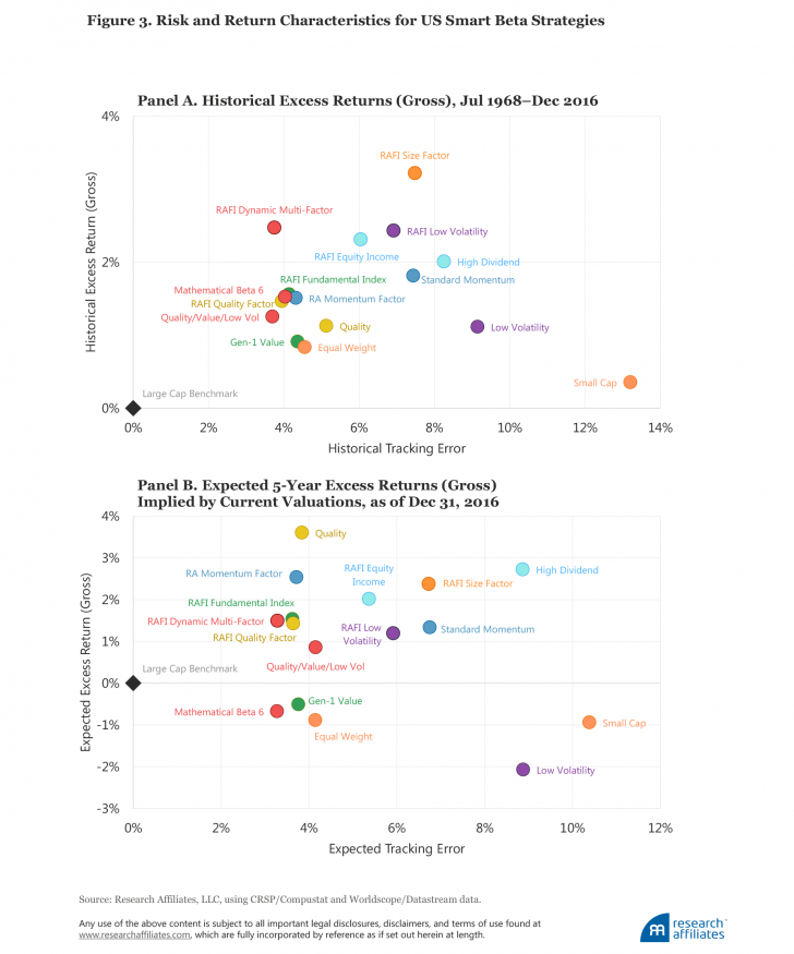
Smart beta strategies with negative forecasted alphas. Like our findings regarding the low beta factor, we project that the low beta and low-volatility strategies will underperform their respective benchmarks across all regions. Even after some pretty disappointing results during the second half of 2016, these strategies still trade at premium valuations. This doesn’t mean that investors should avoid them altogether! They will reduce portfolio volatility and are complementary to many other strategies.

We also project small-cap and equally weighted strategies to have negative returns over the next five years. After a sharp run-up in small versus large stocks during the second half of 2016, the size factor is now expensive relative to average historical valuations in all regions.

Smart beta strategies with positive forecasted alphas. On the other side of the spectrum, strategies with a value orientation, such as the Fundamental Index™, are projected to have high expected returns in most regions.12 Unlike low-volatility or small-cap strategies, value strategies produced only mediocre returns over the last decade, scaring many investors away even though the logic should be the opposite: poor past performance implies cheap valuations, positioning these strategies for healthy performance going forward.

Similarly, income-oriented strategies, such as High Dividend and RAFI™ Equity Income, are generally projected to have high expected returns across all regions. Momentum-oriented strategies in all regions—in stark contrast to a year ago—tend to have decent projected returns, gross of trading costs (which we discuss in the next section).

After faltering rather seriously in the second half of 2016, quality has the highest expected return in the US market, attributable in large degree to its being the mirror image of the B/P value factor. Given the current high level of dispersion in profitability across companies, many high-quality companies are trading at reasonably attractive valuations.

Finally, the RAFI Size Factor strategy is projected to have a much higher return in the US and developed markets than other small cap–oriented strategies. It’s important to note that “RAFI Size Factor” is not the same as the RAFI 1500 for small companies, but rather is a blend of four factor-tilt strategies, each formed within the universe of small-cap stocks: small value, small momentum, small low volatility, and small quality (a factor that combines profitability and investment metrics). Instead of trying to capture the Fama–French SMB (small minus big) factor, one of the factors with weak long-term empirical support, RAFI Size Factor tries to capture other well-documented factor premia within this segment of small stocks having higher risk and higher potential for mispricing.

Trading Costs Matter!

We quants have the luxury of residing in a world of theory and truly vast data. Investors operate in the real world. As such, no discussion of forecast returns would be complete without addressing the costs associated with implementing an investment strategy. All of our preceding analysis—as well as the backtests and simulated smart beta strategy and factor investing performance touted in the market today—deals with paper portfolios.

No fees or trading costs are considered in these paper portfolios, yet in the real world they are a material drag on investors’ performance. Management fees are highly visible and investors are starting to pay a lot more attention to them. We applaud this development. We find it puzzling however that, in order to save a few basis points of visible fees, some investors will eagerly embrace dozens of basis points of trading costs, missed trades, transition costs for changing strategies, and other hidden costs. The impact of these hidden costs is that the investor’s performance is often lower than return forecasts had indicated.13

Monitoring manager performance relative to an index is insufficient to gauge implementation costs. One of the dirty secrets of the indexing world is that indexers can adjust their portfolios for changes in index composition or weights, and changes in the published index take place after these trades have already moved prices. Indexers’ costs per trade can be startlingly high; thankfully, their turnover is generally very low.

Another nuance in assessing “hidden” implementation costs is the impact of related strategies. Investors who index to the Russell 1000 and to the S&P 500 Index have 85–90% overlap in holdings, so they impact each other’s liquidity and trading costs. Another example is the overlap between minimum variance, low volatility, low beta, and low variance strategies, or to cite our own products, the similarity between FTSE RAFI™ and Russell RAFI™. If significant assets are managed under similar strategies, the combined AUM will drive the liquidity and the implementation shortfall of the individual strategies.

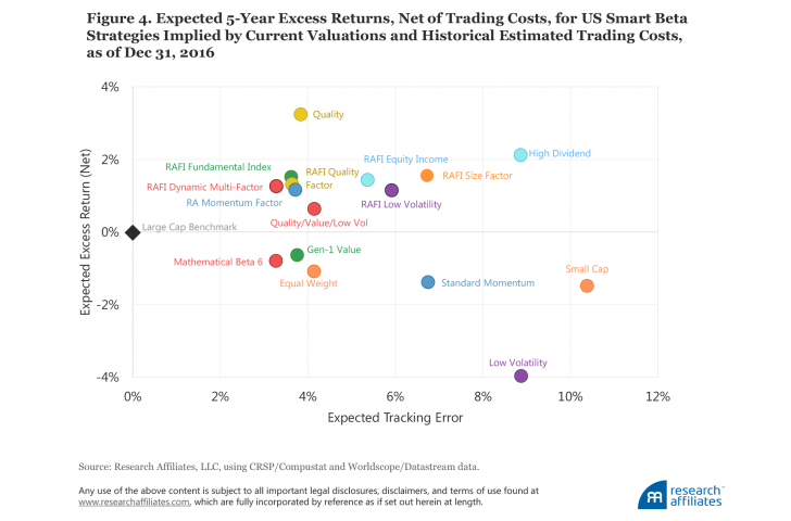
To quantify the effect of trading costs on different strategies we use the model developed by our colleagues Aked and Moroz (2015). The price impact defined by their model is linearly proportional to the amount of trading in individual stocks, measured relative to the average daily volume (ADV). They estimate the price impact is about 30 basis points per each 10% of ADV. For our cost estimates we assume $10 billion is invested in each strategy in the US and developed markets, and $1 billion in the emerging markets. A summary of projected alphas, net of trading costs, in the US market is shown in the scatterplot in Figure 4, as of year-end 2016. The same information for the developed and emerging markets is provided in Appendix E.

Many of the strategies still show quite attractive performance. The heaviest toll from trading costs is on the momentum and low-volatility strategies. Momentum strategies, typified by high turnover and by fierce competition to buy the same stocks at the same time on the rebalancing dates, are likely associated with high trading costs. Low-volatility strategies, already operating from a baseline of low projected returns due to their currently rich valuations, are particularly vulnerable to the impact of trading costs. Low-volatility index calculators and managers should pay close attention to ways to reduce turnover. Again, these strategies have merit for risk reduction and diversification, but we would caution against expecting the lofty returns of the past.

Five-Year Forecasts

We summarize the valuation ratios, historical returns, historical returns net of valuation changes, and expected returns along with estimation errors for the most popular factors and strategies in Table 2. Panel A shows the results for factors, and Panel B shows the results for smart beta strategies. All of these results reflect our method of calculating relative valuation and relative return forecasts, as described in the published methodology for each of these strategies. We caution against acting on these forecasts without examining the potential considerations that our approach doesn’t capture. These forecasts have uncertainty that, in most cases, is larger than the alpha forecast.

Although large, these tables represent only a portion of the multitude of layers and dimensions that investors should consider when evaluating these strategies. We encourage investors and equity managers to use the tables as a reference point when making factor allocation decisions.  As time passes, valuations change, and the expected returns in the table need to be updated to stay relevant. Strategies that seem vulnerable today may be attractively priced tomorrow, and vice versa. The good news is that we will be providing this information, regularly updated, for these and many more strategies and factors on a new interactive section of our website. We encourage readers to visit frequently and to liberally provide feedback.

Putting It All Together

In the brave new “smart beta” world, with the rapid proliferation of factor tilts and quant strategies, investors should be vigilant to the pitfalls of data mining and performance chasing. Our 2016 three-part series covers the topics we believe investors should consider before allocating to such strategies.

In our earlier research, we explained how smart beta can go horribly wrong if investors anchor performance expectations on recent returns. Expecting the past to be prologue sets up two dangerous traps. First, if past performance was fueled by rising valuations, that component of historical performance—revaluation alpha—is not likely to repeat in the future. Worse, we should expect this revaluation alpha to mean revert because strong recent performance frequently leads to poor subsequent performance, and vice versa.

We discussed that winning with smart beta begins by asking if the price is right. Valuations are as important in the performance of factors and smart beta strategies as they are in the performance of stocks, bonds, sectors, regions, asset classes, or any other investment-related category. Starting valuation ratios matter for factor performance regardless of region, regardless of time horizon, and regardless of the valuation metric being used.

We showed how valuations can be used to time smart beta strategies. We know factors can be a source of excess return for equity investors, but that potential excess return is easily wiped out (or worse!) when investors chase the latest hot factor. Investors fare better if we diversify across factors and strategies, with a preference for those that have recently underperformed and are now relatively cheap because of it.

In this article, we offer our estimation of expected returns going forward, based on the logic and the framework we develop in our prior three articles. We hope investors find our five-year forecasts useful in managing expectations about their existing portfolios, and perhaps also in creating winning combinations of strategies, positioned for future—not based on past—success.

Copyright © Research Affiliates