Valuation Based Equity Market Forecasts: Q2 2014

by Adam Butler, http://gestaltu.com

Any analysis that relies on the past to offer guidance about the future makes the strong assumption that the future will in fact resemble the past. We have no guarantee that this will be the case. Many optimistic analysts assert that the invention of central banking, global communications and trade, robotics, 3D printing, Paul Krugman, or any number of ‘game changers’ that have evolved over the past few decades renders comparisons with our past misguided. Surely we won’t make the mistakes of our ancestors; there will be no more war, no misguided political decisions, no shortsighted thinking, no natural disasters, no panics or conflicts or excesses which derail our arc toward ever-increasing prosperity.

In case there is any ambiguity, we do not espouse this Polyanna-esque view. So long as markets, economies and politics are dominated by human judgement, the future is likely to resemble the past in most important respects.

Furthermore, there is, and perhaps always will be, a discussion of whether the stock market is in a ‘bubble’ or whether it is undervalued, overvalued or fairly valued. These labels are meaningless. In reality, markets are always at the ‘right price’ because the entire objective of free markets is to find the clearing price for assets, and the ‘right price’ is the price at which an asset transaction clears between a buyer and a seller. The right price might be higher, from a valuation standpoint, than the historical average implying lower than average future returns, or lower than the historical average implying higher than average future returns. The concepts of ‘right price’ and ‘overvalued’ are not mutually exclusive.

Moreover, we are acutely aware that interest rates are a discounting mechanism and thus low interest rates (especially rates which are expected to remain low for a long time) may justify higher than average equity valuations. This may be a normal condition of asset markets, but it doesn’t alter forecasts about future returns. While markets might be ‘fairly priced’ at high valuations relative to exceedingly low long-term interest rates, this does not change the fact that future returns are likely to be well below average. Again, a market can be ‘fairly priced’ relative to long-term rates, yet still exhibit high valuations implying lower than average future returns. We wouldn’t argue with the assertion that current conditions exhibit these very qualities. However, this fact does not change ANY of the conclusions from the analysis below.

—————————————————————————

We endorse the decisive evidence that markets and economies are complex, dynamic systems which are not reducible to linear cause-effect analysis over short or intermediate time frames. However, the future is likely to rhyme with the past. Thus, we believe there is substantial value in applying simple statistical models to discover average estimates of what the future may hold over meaningful investment horizons (10+ years), while acknowledging the wide range of possibilities that exist around these averages.

To be crystal clear, the commentary below makes no assertions whatsoever about whether markets will carry on higher from current levels. Expensive markets can get much more expensive in the intermediate term, and investors need look no further back than the late 2000s for just such an example. However, the historical implications of investing in expensive markets is that, at some point in the future, perhaps years from now, the market has a very high probability of trading back below current prices; perhaps far below. More importantly, investors must recognize that buying stocks at very expensive valuations will necessarily lead to future returns over the subsequent 10 – 20 years that are far below average.

Many studies have attempted to quantify the relationship between Shiller PE and future stock returns. Shiller PE smoothes away the spikes and troughs in corporate earnings which occur as a result of the business cycle by averaging inflation-adjusted earnings over rolling historical 10-year windows. As discussed above, in this version of our analysis, we have incorporated two new earnings series to address thoughtful concerns raised by other analysts in recent commentaries. We added the Bloomberg series <T12_ESP_AGGTE> and the S&P 500 operating earnings series to account for potentially meaningful changes to GAAP accounting rules in 2001. I would note that Bill Hester at Hussman Funds has addressed this issue comprehensively in a recent report, which we would strongly encourage you to read. Notwithstanding the arguments against using these new series, we felt they offered sufficient merit to include them in our analysis. All CAPE related analyses in this report use a simple average of these three earnings series to calculate the denominator in the CAPE ratio.
[In addition, we reiterate that the final multiple regression model that we use to generate our forecast does not actually include the CAPE ratio as an input. As valuation measures go, this metric is actually less informative than the other three, and reduces the statistical power of the forecast.]
This study also contributes substantially to research on smoothed earnings and Shiller PE by adding three new valuation indicators: the Q-Ratio, total market capitalization to GNP, and deviations from the long-term price trends. The Q-Ratio measures how expensive stocks are relative to the replacement value of corporate assets. Market capitalization to GNP accounts for the aggregate value of U.S. publicly traded business as a proportion of the size of the economy. In 2001, Warren Buffett wrote an article in Fortune where he states, “The ratio has certain limitations in telling you what you need to know. Still, it is probably the best single measure of where valuations stand at any given moment.” Lastly, deviations from the long-term trend of the S&P inflation adjusted price series indicate how ‘stretched’ values are above or below their long-term averages.
These three measures take on further gravity when we consider that they are derived from four distinct facets of financial markets: Shiller PE focuses on the earnings statement; Q-ratio focuses on the balance sheet; market cap to GNP focuses on corporate value as a proportion of the size of the economy; and deviation from price trend focuses on a technical price series. Taken together, they capture a wide swath of information about markets.
We analyzed the power of each of these ‘valuation’ measures to explain inflation-adjusted stock returns including reinvested dividends over subsequent multi-year periods. Our analysis provides compelling evidence that future returns will be lower when starting valuations are high, and that returns will be higher in periods where starting valuations are low.

Again, we are not making a forecast of market returns over the next several months; in fact, markets could go substantially higher from here. However, over the next 10 to 15 years, markets are very likely to revert to average valuations, which are much lower than current levels. This study will demonstrate that investors should expect 6.5% real returns to stocks only during those very rare occasions when the stock market passes through ‘fair value’ on its way to becoming very cheap, or very expensive. At all other periods, there is a better estimate of future returns than the long-term average, and this study endeavors to quantify that estimate.

Investors should be aware that, relative to meaningful historical precedents, markets are currently expensive and overbought by all measures covered in this study, indicating a strong likelihood of low inflation-adjusted returns going forward over horizons of 10-20 years.
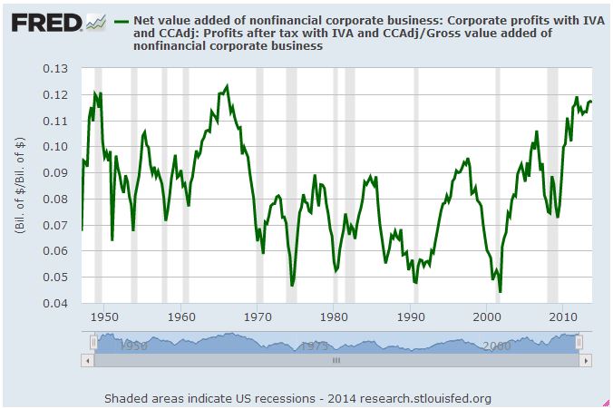
This forecast is also supported by evidence from an analysis of corporate profit margins. In a recent article, Jesse Livermore at Philosophical Economics published a long-term chart of adjusted U.S. profit margins, which demonstrates the magnitude of upward distortion endemic in current corporate profits, which we have reproduced in Chart 1 below. Companies have clearly been benefiting from a period of extraordinary profitability.
Chart 1. Inflated U.S. adjusted profit margins
nonfincp

 Source: Philosophical Economics, 2014

The profit margin picture is critically important. Jeremy Grantham recently stated, “Profit margins are probably the most mean-reverting series in finance, and if profit margins do not mean-revert, then something has gone badly wrong with capitalism. If high profits do not attract competition, there is something wrong with the system and it is not functioning properly.” On this basis, we can expect profit margins to begin to revert to more normalized ratios over coming months. If so, stocks may face a future where multiples to corporate earnings are contracting at the same time that the growth in earnings is also contracting. This double feedback mechanism may partially explain why our statistical model predicts such low real returns in coming years. Caveat Emptor.

Modeling Across Many Horizons

Many studies have been published on the Shiller PE, and how well (or not) it estimates future returns. Almost all of these studies apply a rolling 10-year window to earnings as advocated by Dr. Shiller. But is there something magical about a 10-year earnings smoothing factor? Further, is there anything magical about a 10-year forecast horizon?
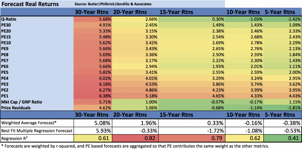
Table 1. below provides a snapshot of some of the results from our analysis. The table shows estimated future returns based on a coherent aggregation of several factor models over some important investment horizons.
Table 1. Factor Based Return Forecasts Over Important Investment Horizons
Forecast_Summary
Source: Shiller (2013), DShort.com (2013), Chris Turner (2013), World Exchange Forum (2013), Federal Reserve (2013), Butler|Philbrick|Gordillo & Associates (2013)
You can see from the table that, according to a model that incorporates valuation estimates from 4 distinct domains, and which explains over 80% of historical returns since 1928, stocks are likely to deliver less than 0% in real total returns over the next 5 to 20 years. Budget accordingly.

Process

The purpose of our analysis was to examine several methods of capturing market valuation to determine which methods were more or less efficacious. Furthermore, we were interested in how to best integrate our valuation metrics into a coherent statistical framework that would provide us with the best estimate of future returns. Our approach relies on a common statistical technique called linear regression, which takes as inputs the valuation metrics we calculate from a variety of sources, and determines how sensitive actual future returns are to contemporaneous observations of each metric.
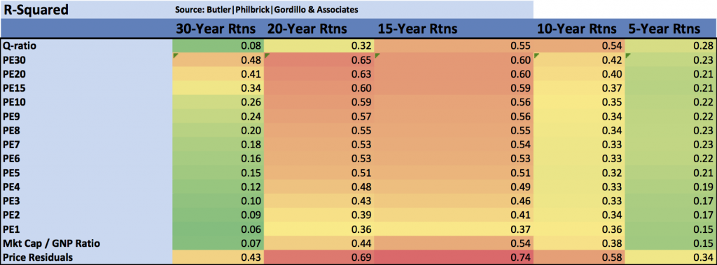
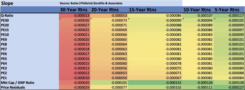
Linear regression creates a linear function, which by definition can be described by a slope value and an intercept value, which we provide below for each metric and each forecast horizon. A further advantage of linear regression is that we can measure how confident we can be in the estimate provided by the analysis. The quantity we use to measure confidence in the estimates is called the R-Squared. The following matrices show the R-Squared ratio, regression slope, regression intercept, and current forecast returns based on a regression analysis for each valuation factor. The matrices are heat-mapped so that larger values are reddish, and small or negative values are blue-ish. Click on each image for a large version.
Matrix 1. Explanatory power of valuation/future returns relationships
r_squared_matrix
Source: Shiller (2014), DShort.com (2014), Chris Turner (2014), World Exchange Forum (2014), Federal Reserve (2014), Butler|Philbrick|Gordillo & Associates (2014)
Matrix 1. contains a few important observations. Notably, over periods of 10-20 years, the Q ratio, very long-term smoothed PE ratios, and market capitalization / GNP ratios are equally explanatory, with R-Squared ratios around 55%. The best estimate (perhaps tautologically given the derivation) is derived from the price residuals, which simply quantify how extended prices are above or below their long-term trend. The worst estimates are those derived from trailing 12-month PE ratios (PE1 in Matrix 1 above). Many analysts quote ‘Trailing 12-Months’ or TTM PE ratios for the market as a tool to assess whether markets are cheap or expensive. If you hear an analyst quoting the market’s PE ratio, odds are they are referring to this TTM number. Our analysis slightly modifies this measure by averaging the PE over the prior 12 months rather than using trailing cumulative earnings through the current month, but this change does not substantially alter the results. As it turns out, TTM (or PE1) Price/Earnings ratios offer the least information about subsequent returns relative to all of the other metrics in our sample. As a result, investors should be extremely skeptical of conclusions about market return prospects presented by analysts who justify their forecasts based on trailing 12-month ratios.

Forecasting Expected Returns

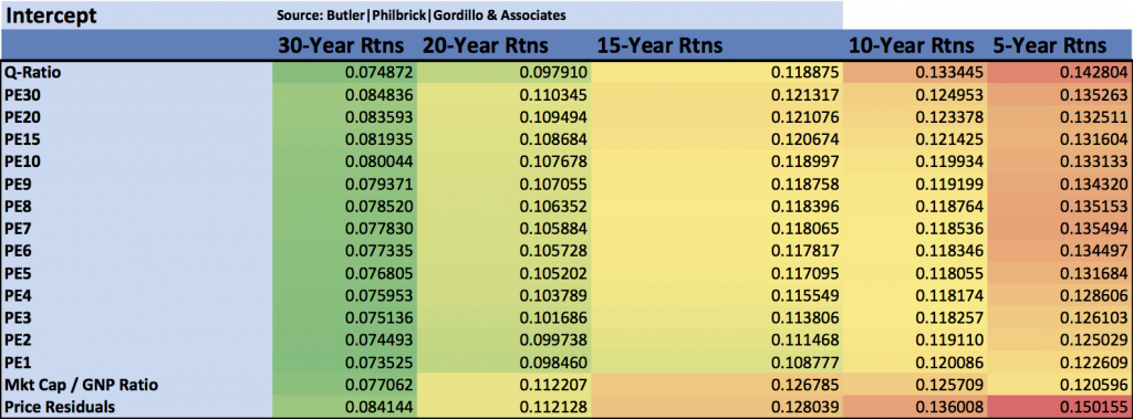
We expect you to be skeptical of our unconventional assertions, so below we provide the precise calculations we used to determine our estimates. The following matrices provide the slope and intercept coefficients for each regression. We have provided these in order to illustrate how we calculated the values for the final matrix below of predicted future returns to stocks.
Matrix 2. Slope of regression line for each valuation factor/time horizon pair.
Slope_Matrix
Source: Shiller (2014), DShort.com (2014), Chris Turner (2014), World Exchange Forum (2014), Federal Reserve (2014), Butler|Philbrick|Gordillo & Associates (2014)
Matrix 3. Intercept of regression line for each valuation factor/time horizon pair.
Intercept_Matrix
Source: Shiller (2014), DShort.com (2014), Chris Turner (2014), World Exchange Forum (2014), Federal Reserve (2014), Butler|Philbrick|Gordillo & Associates (2014)
Matrix 4. shows forecast future real returns over each time horizon, as calculated from the slopes and intercepts above, by using the most recent values for each valuation metric (through June 2014). For statistical reasons which are beyond the scope of this study, when we solve for future returns based on current monthly data, we utilize the rank in the equation for each metric, not the nominal value. For example, the 15-year return forecast based on the current Q-Ratio can be calculated by multiplying the current ordinal rank of the Q-Ratio (1343) by the slope from Matrix 2. at the intersection of ‘Q-Ratio’ and ’15-Year Rtns’ (-0.000086), and then adding the intercept at the same intersection (0.118875) from Matrix 3. The result is 0.003, or 0.30%, as you can see in Matrix 4. below at the same intersection (Q-Ratio | 15-Year Rtns).
Matrix 4. Modeled forecast future returns using current valuations.
Forecast_Matrix1
Source: Shiller (2014), DShort.com (2014), Chris Turner (2014), World Exchange Forum (2014), Federal Reserve (2014), Butler|Philbrick|Gordillo & Associates (2014)
Finally, at the bottom of the above matrix we show the forecast returns over each future horizon based on a weighted average of all of the forecasts, and again by our best-fit multiple regression from the factors above. From the matrix, note that forecasts for future real equity returns integrating all available valuation metrics are less than 2% per year over horizons covering the next 5 to 20 years. We also provide the R-squared for each multiple regression underneath each forecast; you can see that at the 15-year forecast horizon, our regression explains over 80% of total returns to stocks.
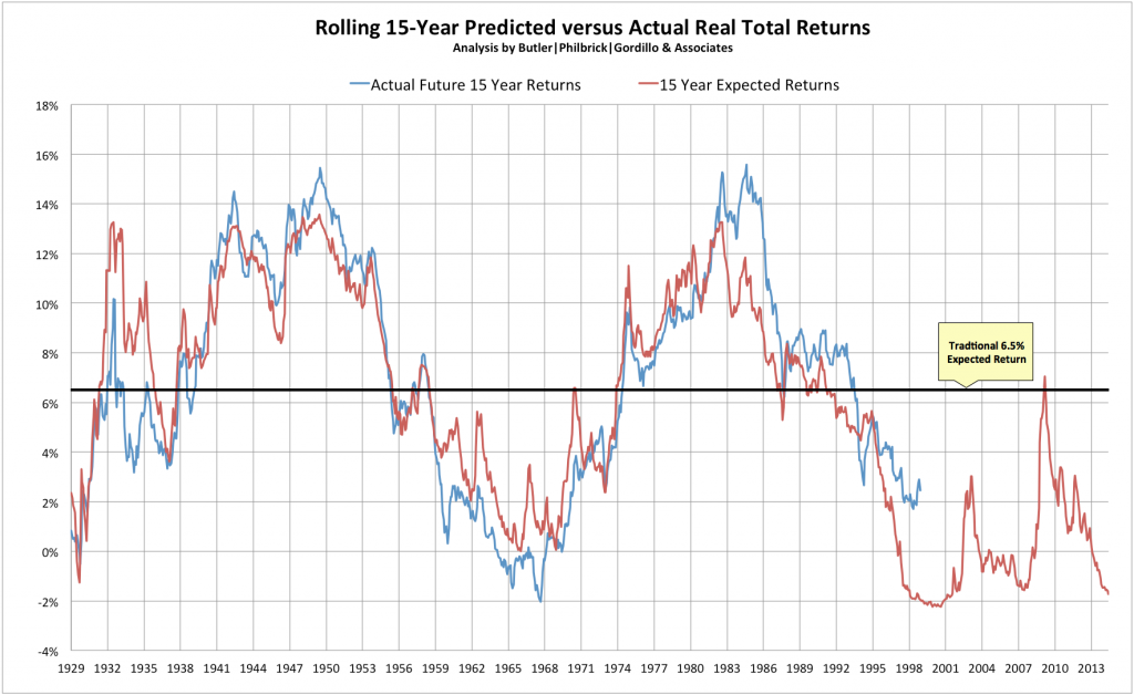
Chart 2. below demonstrates how closely the model tracks actual future 15-year returns. The red line tracks the model’s forecast annualized real total returns over subsequent 15-year periods using our best fit multiple regression model . The blue line shows the actual annualized real total returns over the same 15-year horizon.

Chart 2. 15-Year Forecast Returns vs. 15-Year Actual Future Returns
Chart
Source: Shiller (2014), DShort.com (2014), Chris Turner (2014), World Exchange Forum (2014), Federal Reserve (2014)

Putting the Forecasts to the Test

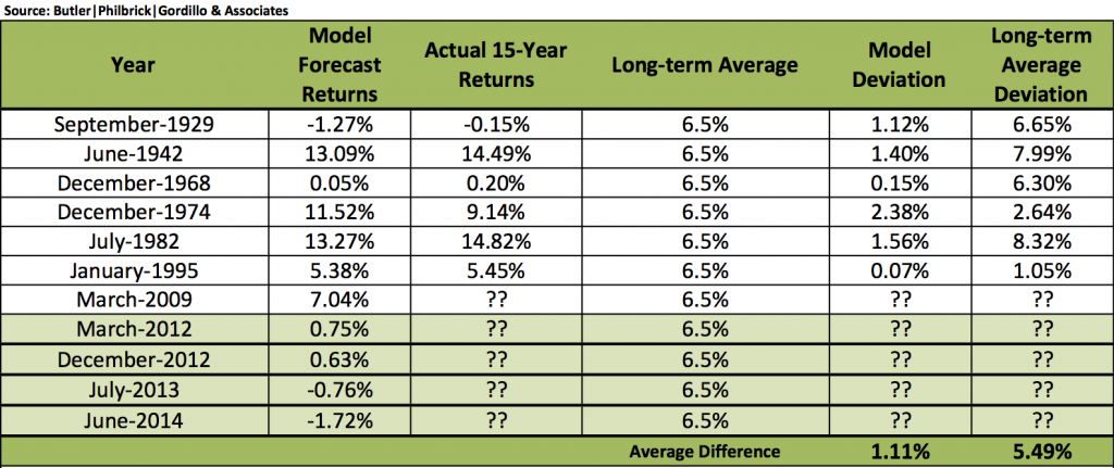
A model is not very interesting or useful unless it actually does a good job of predicting the future. To that end, we tested the model’s predictive capacity at some key turning points in markets over the past century or more to see how well it predicted future inflation-adjusted returns.
Table 2. Comparing Long-term average forecasts with model forecasts
Examples_Matrix
Source: Shiller (2014), DShort.com (2014), Chris Turner (2014), World Exchange Forum (2014), Federal Reserve (2014), Butler|Philbrick|Gordillo & Associates (2014)
You can see we tested against periods during the Great Depression, the 1970s inflationary bear market, the 1982 bottom, and the middle of the 1990s technology bubble in 1995. The table also shows expected 15-year returns given market valuations at the 2009 bottom, and current levels. These are shaded green because we do not have 15-year future returns from these periods yet. Observe that, at the very bottom of the bear market in 2009, real total return forecasts never edged higher than 7%, which is only slightly above the long-term average return. This suggests that prices just approached fair value at the market’s bottom; they were nowhere near the level of cheapness that markets achieved at bottoms in 1932 or 1982. As of the end of June 2014, annualized future returns over the next 15 years are expected to be less than zero percent.
We compared the forecasts from our model with what would be expected from using just the long-term average real returns of 6.5% as a constant forecast, and demonstrated that always using the long-term average return as the future return estimate resulted in 500% more error than estimations from our multi-factor regression model over 15-year forecast horizons (1.11% annualized return error from our model vs 5.49% using the long-term average). Clearly the model offers substantially more insight into future return expectations than simple long-term averages, especially near valuation extremes (dare we say, like we observe today?)

Conclusions

The ‘Regression Forecast’ return predictions along the bottom of Matrix 4. are robust predictions for future stock returns, as they account for over 100 different cuts of the data, using 4 distinct valuation techniques, and utilize the most explanatory statistical relationships. Notwithstanding the statistical challenges described above related to overlapping periods, the models explain a meaningful portion of future returns. Despite the model’s robustness over longer horizons, it is critical to note that even this model has very little explanatory power over horizons less than 6 or 7 years, so the model should not be used as a short-term market-timing tool.
Returns in the reddish row labeled “PE1″ in Matrix 4 were forecast using just the most recent 12 months of earnings data, and correlate strongly with common “Trailing 12-Month” PE ratios cited in the media. Matrix 1. demonstrates that this trailing 12 month measure is not worth very much as a measure for forecasting future returns over any horizon. However, the more constructive results from this metric probably helps to explain the general consensus among sell-side market strategists that markets will do just fine over coming years. Just remember that these analysts have no proven ability whatsoever to predict market returns (see here, here, and here). This reality probably has less to do with the analytical ability of most analysts, and more to do with the fact that most clients would choose to avoid investing in stocks altogether if they were told to expect negative real returns over the long-term from high valuations.
Investors would do much better to heed the results of robust statistical analyses of actual market history, and play to the relative odds. This analysis suggests that markets are currently expensive, and asserts a very high probability of low returns to stocks (and possibly other asset classes) in the future. Remember, any returns earned above the average are necessarily earned at someone else’s expense, so it will likely be necessary to do something radically different than everyone else to capture excess returns going forward. Those investors who are determined to achieve long-term financial objectives should be heavily motivated to seek alternatives to traditional investment options given the grim prospects outlined above. Such investors may find solace in some of the approaches related to ‘tactical alpha’ that we have described in a variety of prior articles.
————————————————–
Considerations & Next Steps

We first published a valuation based market forecast in September of 2010. At that time we used only the Shiller PE data to generate our forecast, and our analysis suggested investors should expect under 5% per year after inflation over the subsequent 10 year horizon. Over the 40 months since we have introduced several new metrics and applied much more comprehensive methods to derive our forecast estimates. Still, our estimates are far from perfect.

From a statistical standpoint, the use of overlapping periods substantially weakens the statistical significance of our estimates. This is unavoidable, as our sample only extends back to 1900, which gives us only 114 years to work with, and our research suggests that secular mean reversion exerts its strongest influence on a periodicity somewhere between 15 and 20 years. As a result, our true sample size is somewhere between 5 and 6, which is not very high. 

Aside from statistical challenges, readers should consider the potential for issues related to changes in the way accounting identities have been calculated through time, changes to the geographic composition of earnings, and myriad other factors. For a comprehensive analysis of these challenges we encourage readers to visit the Philosophical Economics (PE) blog.

It should be noted that, while we recommend readers take the time to consider the comprehensive analyses published by Philosophical Economics over the past few months, we are rather skeptical of some of the author’s more recent assertions. In particular, we challenge the notion that model errors related to dividends, growth and valuations are independent of one another, and can therefore be disaggregated in the way the author presents. Dividend yields and earnings growth are inextricably and causally related to each other (lower dividend payout ratios are causally related to stronger future earnings growth because of higher rates of reinvestment, and vice versa), thus we would expect them to have inverse cumulative error terms. The presence of such inverse error terms simply proves this causal link empirically, and offers no meaningful information about the validity of valuation based reversion models.

We also take grave issue with the contention that the valuation-based reversion observed in stocks over periods of 10 years (which Hussman uses) should be dismissed as ‘curve fitting’. According to PE, since we observe some reversion over 10 year periods we should observe the same or stronger reversion over a 30 year horizon, because 30 years is a multiple of 10 years. But the author discovers virtually no explanatory relationship at 30 year reversion horizons. From this observation he concludes that valuation-based mean-reversion at the 10 year horizon is invalid, and that the 10 year reversion relationship is a curve-fit aberration with no statistical significance. 

The logical flaw in this argument is revealed by an examination of our own results. Our analysis suggests markets exhibit most significant mean reversion at periods of 15 to 20 years (though 10 years is still significant). This suggests that markets will have completed a full cycle (that is, will have come ‘full circle’) after 30 or 40 years. In other words, if markets are currently expensive, then 15 or 20 years from now they will probably be cheap. Of course, 15 or 20 years on from that point (or 30 to 40 years from now) markets will have returned to their original expensive condition. Thus no mean-reversion relationship will be observed over 30-40 years. Any analyses of mean reversion over periods of 30 or 40 years will not find any relationship because cheap prices will have passed through expensive prices and gone back to cheap over the span of the full cycle. 

In case this is still unclear, consider a similar concept in a related domain: stock momentum. Eugene Fama, the father of ‘efficient markets’ described the momentum anomaly in equities as ‘the premier unexplained anomaly’, yet it only works at a frequency of about 2 to 12 months; that is, if you buy a basket of stocks that had the greatest price increase over the prior 2 to 12 month period, those stocks are likely to be among the top performers over the next few weeks or months. However, momentum measured over a 3 to 5 year period works in precisely the opposite manner: the worst performing stocks over the past 3 to 5 years generate the strongest returns. Now, 3 and 5 years are multiples of 12 months, yet extending the analysis to multiples of the 12 month frequency delivers the exact opposite effect. Should we dismiss the momentum anomaly as curve fitting then?

Eugene Fama doesn’t think so, and neither do we.

That said, we see value in the questions PE raised about the changing nature of earnings series and margin calculations. Largely driven PE’s analysis, we integrated new earnings series from Bloomberg and S&P into our Cyclically Adjusted PE calculation for model calculations. Primarily, the new series adjust earnings for changes to GAAP rules in 2001 related to corporate write-downs. Each of the series has merit, so we took the step of averaging them without prejudice. I’m sure bulls and bears alike will find this method unsatisfying; we certainly hope so, as the best compromises have this precise character.

Importantly, the new earnings series do not alter the final regression forecast model results because our multiple regression model rejects the Shiller PE as statistically insignificant to the forecast. That is, it is highly collinear with, but less significant than, other series like market cap/GNP and q ratio. This has been the case from the beginning of this article series, so it isn’t due to the new earnings data. Nevertheless we include regression parameters and r-squared estimates for all of the modified Shiller PEs in the matrices as usual.

The bottom line is that, despite statistical and accounting challenges, our indicators have proved to be of fairly consistent value in identifying periods of over and under-valuation in U.S. markets over about a century of observation, notwithstanding the last two decades. We admit that the two decades since 1994 seem like strange outliers relative to the other seven decades; history will eventually prove whether this anomaly relates to a structural change in the calculation of the underlying valuation metrics, a regime shift in the range of possible long-term returns, an increase in the ambient slope of drift, or something as of yet entirely unconsidered.

We all must acknowledge that the current globally coordinated monetary experiment truly has no precedent in modern history. For this reason the range of potential outcomes is much wider than it might otherwise be. Things could persist for much longer, and reach never before seen extremes (in both directions, mind you!) before it’s over.

Lastly, I am struggling to reconcile a conundrum I identified very early in the development of our multi-factor model. Namely, the fact that the simple regression of real total returns with reinvested dividends carries very different implications than the suite of other indicators we have tested. Georg Vrba explores this model in some detail, and we recommend readers take a moment to consider his views in this domain. I am troubled by the theoretical veracity of incorporating dividend reinvestment for extrapolation purposes, because the vast majority of dividends are NOT reinvested, but rather are paid out, and represent a material source of total income in the economy. However, the trend fit is surprisingly tight, and I can’t say with conviction that the model is any less valid than the other methods we apply in this analysis. It is a puzzle.

The bottom line is that as researchers, we deeply appreciate respectful disagreements. This is because there are only three possible outcomes for the introduction of new and contrary evidence into a discussion. First, it could prove worthy of inclusion, improving the accuracy and timeliness of estimates. The inclusion of new earnings series is an excellent example of this, as we’ve been convinced by the evidence presented by Jesse Livermore in this domain. Second, it could prove unworthy of inclusion, which we can only know upon stress-testing our model, thereby increasing our confidence in its reliability. The rejection of the notion that valuation-based reversion is curve-fitting would be such an example. Or third, it could provoke a ‘deep dive’ that evolves into a complete overhaul of current models, and/or an interesting future research publication. Vrba’s dividend reinvestment notion is a prominent member of this category.

We thank everyone – on all sides of the debate – for their continued contributions (either explicitly or implicitly) to the ongoing evolution of this research.

The post Valuation Based Equity Market Forecasts: Q2 2014 appeared first on GestaltU.

Source link

Total
0
Shares
Previous Article

10 Painfully Obvious Truths Everyone Forgets Too Soon, and other Weekend Reads

Next Article

This Might be a Stock Bubble, but Valuation Metrics Won’t Help you Understand That

Related Posts
Subscribe to AdvisorAnalyst.com notifications
Watch. Listen. Read. Raise your average.