Deborah Frame: Why Do We Accept Volatility as a Measure of Risk?

Not Your Grandfather’s Risk Measurement

by Deborah Frame, Vice President, Investments, Cougar Global Investments

Why Do We Accept Volatility as a Measure of Risk? — Recognizing the Non-Normality of Asset Class Returns

When you ask an individual what they regard as risk when it comes to their investment exposure, the vast majority answer “losing money”. They have no problem with unexpected high rates of return but they do have a problem with seeing their capital eroded. This is not the same as risk measured as volatility. Some very good articles regarding risk in today’s markets and in portfolio construction have addressed the flaws of looking at volatility as a risk measure. This granular look is premised on the axiom that it is the contributors to volatility, rather than the idea of volatility as a risk measure itself that needs to be understood.

To outright reject volatility as a measure of risk, we need to understand what is being measured, monitored and constraining portfolio asset allocation in institutional investment management today. The work of Harry Markowitz in the late 1950s and early 1960s has left a heavy stamp on this aspect of portfolio management from that time up to this day. The thinking goes like this.Asset classes experience a large distribution of returns over time, typically ranging from losses to returns far in excess of the average return, calculated over the measurement period. Markowitz defined both upside and downside deviation from a mean – mean variance or “volatility” as risk and assumed that losses always exactly equalled gains- the “normal curve”. Until recently, investors have been constrained in their ability to incorporate the true asymmetrical distribution of returns or “non-normality” into the asset allocation process. But now, with the availability of sophisticated statistical tools and modern computing power, we do not need to settle for this simplifying assumption of fifty years ago and can meet the challenge of isolating the probability of suffering losses.

Why is rejecting Markowitz’s volatility and embracing non-normality the key to successful portfolio management?

The most straightforward answer is that this is how the world really works—i.e. we empirically observe non-normality with much greater frequency than the more entrenched mean-variance frameworks allow for. But more importantly, ignoring non-normality in equity (and equity type) return distributions significantly understates downside portfolio risk - losses.

Macro-economic environments result in the incidence of non-normality of asset class return distributions. This, along with the recognition of greater downside risk to asset classes from periodic extreme unexpected negative events and changing economic environments can be incorporated into tactical asset allocation driven portfolio models and delivered with an optimal combination of broad asset class Exchange Traded Funds (ETFs).

How can this be done? An investment manager (my firm-Cougar Global Investments) can consider the outlook for the global economy and bring it back to a view of expected US GDP growth in the twelve months ahead. The outlook falls into one of the following five broad descriptions : GROWTH, STAGNATION, RECESSION, INFLATION and CHAOS but allows for the possibility of a transitioning in the period from one environment to another. Historical asset class monthly return data is tagged using rules to assign each month with one of the five environments. We have modelled over thirty asset classes. From this tagging, expected return distributions are created by drawing return data using boot-stapping (random sampling with replacement) from past economic environments that are similar to what is anticipated in the coming twelve months. The twelve month forward outlook and updating of expected return distributions is updated monthly.

Much has been written about the randomness of asset class behaviour over time, both in terms of returns and correlations to other asset classes. As studies on what drives the returns of asset classes have identified, the macro -economic environment factors into returns but the contribution is not static, its significance changes over time and is different among different asset classes. Remarkably, when historic data for asset classes is partitioned under broad economic environments, patterns of behaviour become obvious. This allows portfolios to be created with ETFs that are the closest proxy to the asset classes that are used in the modelling process. Using ETFs we can specifically address expected returns among the asset classes being considered while also addressing the probability of negative returns in those asset classes in the anticipated economic environment.

The Asset Class Examples

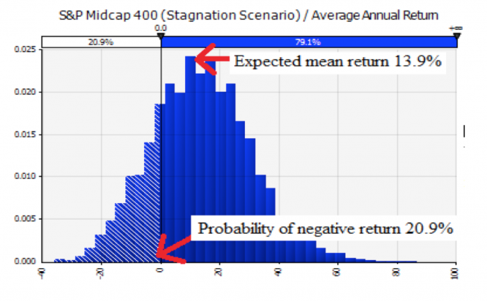
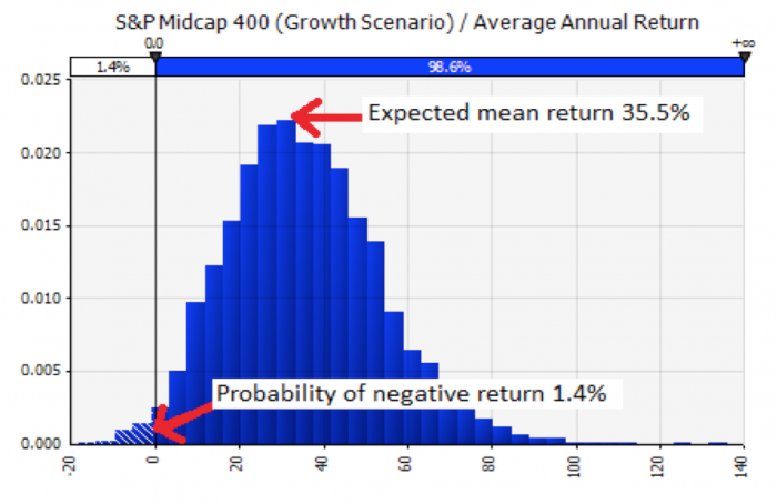
A good equity index example is the S&P 400 Mid Cap Index. In Stagnation the current bootstrapped expected return distribution indicates an expected mean return of 13.9% with a probability of going negative of 20.9%. In Growth the expected mean return is 35.5% and the probability of going negative is 1.4%. . This exercise indicates that we can expect a higher return with a lower probability of experiencing a loss as we move from Stagnation to Growth. The SPDR S&P MidCap 400 ETF (MDY) can be used to get this exposure in an ETF portfolio.

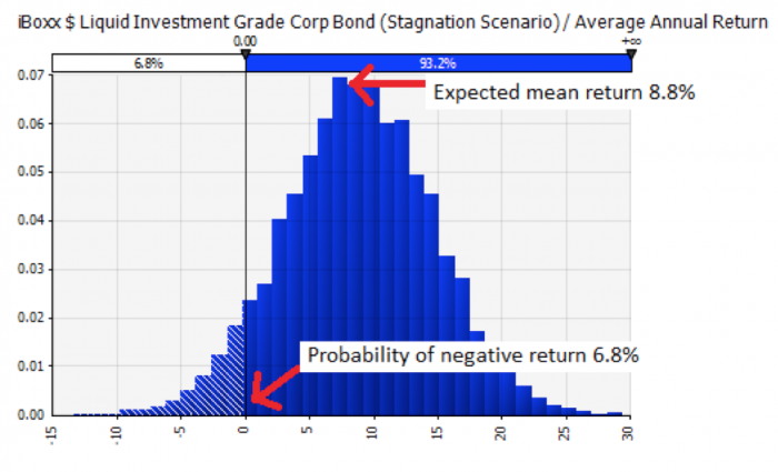
Using the same historical data set, the Iboxx Investment Grade Corporate Bond Index shows a bootstrapped expected mean return in Stagnation of 8.8% and a probability of going negative of 6.8%. In Growth the expected mean falls to 5.4% and the probability of going negative increases to 20.2%. The conclusion here is that we can expect a lower return and higher probability of experiencing a loss for the Iboxx Investment Grade Corporate Bond as we move from Stagnation to Growth. In this simple example the portfolio optimizer will prefer more of the S&P 400 Mid Cap Index and less of the Iboxx Investment Grade Corporate Bond as we move from Stagnation to Growth. The iShares iboxx Investment Grade Corporate ETF (LQD) can be used to get this exposure in an ETF portfolio.

Of course the past will never be exactly repeated in the future. And with exogenous stimulative monetary policy like Quantitative Easing promoting growth behaviour in equity asset classes while the underlying economy has been languishing over the past three years and until very recently in stagnation, a certain amount of adaptability must be introduced when using return data from previous environments. The purpose here is more to highlight the benefits of a tactical approach centred on the significance of the macro-economic environment to downside risk management using ETFs.

Fortunately, this tactical approach which combines the qualitative judgement required when considering the economic environment over the coming twelve months with the quantitative preciseness of bootstrapping and optimization has produced portfolios over the past twenty years that have demonstrated that there can be success in any market or economic environment.

With an awareness of asset class correlations- relative behaviour in changing macro- economic environments, the idea of maintaining a locked-in 60 percent in equities and 40 percent in fixed income that grew from the Markowitz view of risk as volatility becomes unnecessary and a liability to long-term successful investing.

Deborah Frame
Vice President Investments
Cougar Global Investments

Copyright © Cougar Global Investments