Reading the Right Tea Leaves to Gauge Market Volatility

by Daniel Morillo, Ph. D., iShares

Investors have become all too familiar with volatility in recent years as dramatic events like the Lehman Brothers bankruptcy and the downgrade of US debt have rattled global markets. Last month, my colleague Russ Koesterich said in a blogthat he expects volatility to remain elevated for the remainder of the decade.

That call might seem quite bold given the difficulty in predicting the type of individual events that tend to trigger volatility in the markets. But Russ wasn’t reacting to short-term events when he wrote that post. Instead, he was focused on underlying trends that could influence longer-term behavior of the markets. Why? Well, over extended periods of time, market volatility has been linked to uncertainty in broad macroeconomic prospects and not the latest breaking news headline.

There is a large body of academic literature that explores this link. But I’d like to illustrate this relationship using two simple macroeconomic metrics – economic growth and changes in the money supply.

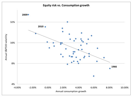
First, let’s look at economic growth. Poor economic growth makes investment planning generally more difficult and more sensitive to specific market, political or policy events. As the chart below shows, since the 1960s US consumption growth (or lack thereof) has accounted for about 30% of the variation in annual volatility for the S&P 500 index[1]. In other words, the more consumption growth, the lower volatility and vice versa.

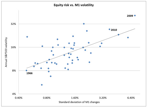
Now, let’s look at the volatility in changes to the money supply. “Narrow” money supply or M1 is the total amount of currency, checking and other liquid deposits in banks and other financial institutions across the economy. This metric is useful because the total amount of liquid instruments such as cash and bank deposits that investors and consumers hold is very sensitive to expectations about interest rates and credit conditions, which are the key targets of monetary policy. Since 1960, volatility in M1 changes explains close to 40% of the annual variation in S&P 500 volatility[2].

When combined, these two metrics can explain around half of the annual variation in S&P 500 volatility. That is a very large amount given the simplicity of the metrics used and the fact that they apply to more than 50 years of US equity market history. This makes simple, high-level scenario analysis for volatility reasonably straightforward[3] and explains why it is important for investors to look beyond short-term events.

In this case, low consumption growth (defined as the 25th percentile of consumption growth over the last 50 years, or annual consumption growth around 2% or less) and high money supply volatility (defined as the 75th percentile of M1 volatility over the last 50 years) would be associated with around 18% annual volatility over the next two to three years. That is well above the 13% annual volatility that is the median observed in the last 50 years of history.

This simple scenario analysis suggests investors should plan for an extended period of higher-than-normal volatility, independent of any specific views about the likely outcome of European debt crisis, US elections and other near-term events. A well-diversified portfolio, including strategies that seek stability in periods of high-volatility such as minimum volatility strategies, should be near the top of the list for investors to consider as they plan their long-term investments.

Daniel Morillo, PhD is the iShares Head of Investment Research and a regular contributor to the iShares Blog. You can find more of his posts here.

Diversification and minimum volatility strategies may not protect against market risk.

[1] Volatility is measured for every year since 1960 as the annualized standard deviation in S&P500 daily returns. Data for S&P500 returns is from Bloomberg. Consumption growth is measured as the real annual growth as reported in the FRED database.
[2] M1 data is obtained in monthly frequency from the FRED database. M1 changes are computed as month-to-month percentage changes. M1 volatility is computed as the annualized standard deviation of the monthly changes.

[3] Scenario analysis is done using a simple linear regression of annual volatility on the two metrics described for the full 1960-2011 period. Volatility and M1 change volatility are used in logs, as is standard practice.

Copyright © iShares