Stop the Losses!

by Jay Jeon & Jim Masturzo, Research Affiliates

Key Points

• Even thoughtfully managed strategies may underperform or suffer sharp losses. This can encourage poorly timed emotional decisions that exacerbate the decline. A systematic risk-management framework that employs stop losses can help minimize such behavioral biases.
• Stop losses are a critical risk-management tool for many portfolio approaches, including alternative risk premia and trend-following strategies, that capture systematic sources of return but often fail to define rules that can provide protection during extreme market events when historical patterns break down.
• The right level of protection, through appropriate stop-loss levels, depends on each strategy’s needs and must balance improved risk characteristics against the reduction in risk-adjusted returns (Sharpe ratio).
• With simple signals and basic portfolio construction methods, stop losses can decrease skewness and drawdowns for both alternative risk premia and trend-following strategies.

Jim Masturzo is the corresponding author.

The Risks of Systematic Strategies

In the age of machine learning and artificial intelligence (AI), an ever-increasing number of managers are constructing complex signals and risk models to include in their portfolios. However, even the most carefully crafted signals may suffer periods of underperformance, and dependable correlation and volatility models can fail during times of elevated uncertainty. This leads to outsized positions that may expose a strategy to potentially catastrophic risks.

To illustrate this point, consider alternative risk premia (ARP) strategies. These come down to two choices, what risk premia (signals) to harvest and what risks (risk factors) to hedge. In Jeon and Masturzo (2024), we discuss the importance of mitigating unintended risk-factor exposures when constructing ARP strategies. Our process lays out a foundation for building ARP portfolios; however, no process is perfect for all market environments, and there is always more to consider.

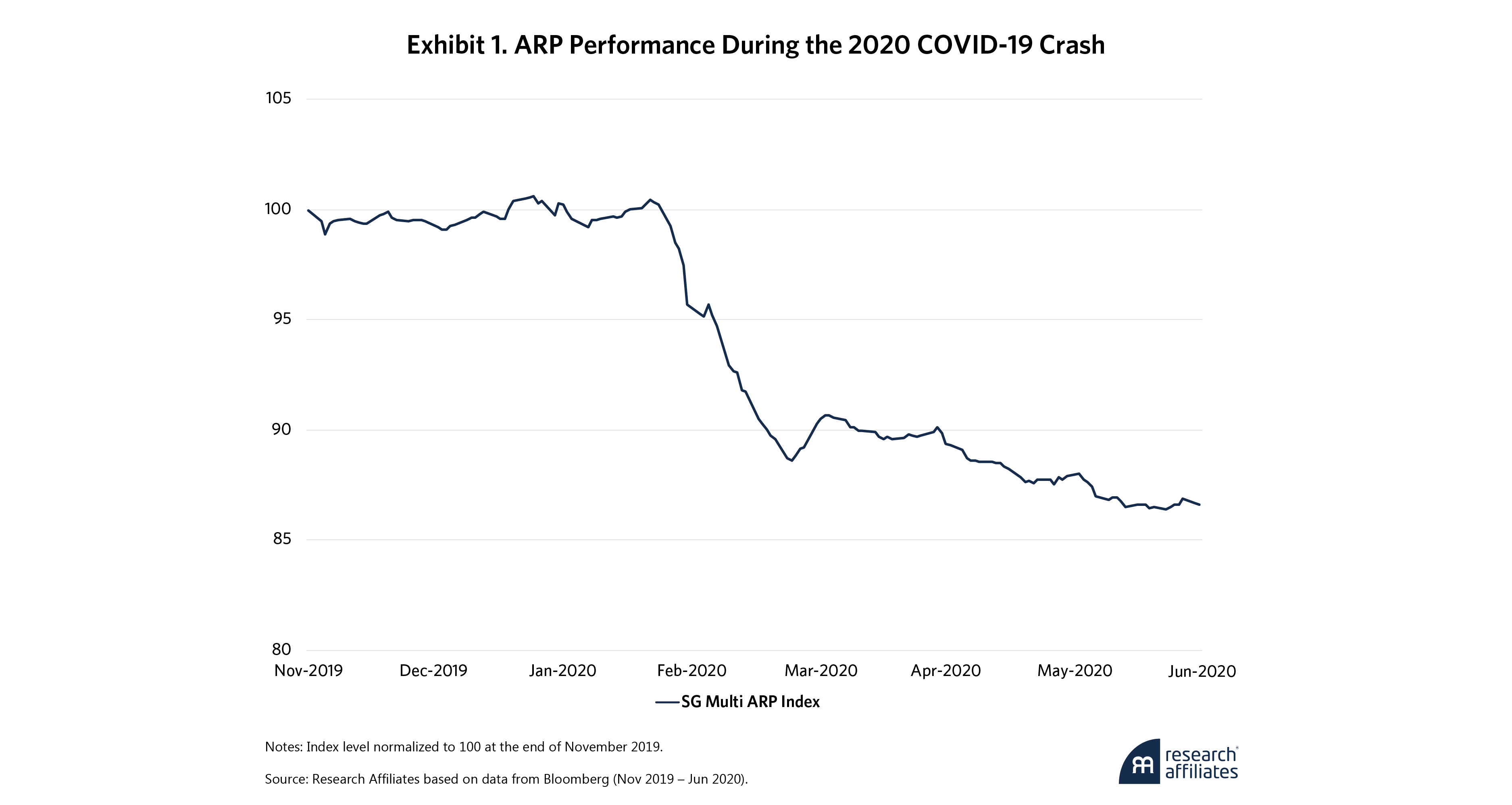
Recall the tumult when COVID-19’s impacts began to materialize around the globe. Investors fled to safety, causing broad, double-digit equity market crashes. How did low-beta ARP strategies perform during these times? As Exhibit 1 shows, not very well. The SG Multi Alternative Risk Premia Index, comprised of various ARP funds, fell more than 10% in March 2020. To put that in perspective, the index’s trailing one-year volatility, from March 2019 to February 2020, was only 4.4%. It is doubtful this reflected these strategies’ desired risk profiles.

What happened? It’s difficult to say without knowing the inner workings of the funds that compose the index, but at a high level, it probably had something to do with the breakdown of the historical relationships on which these strategies relied. Whether correlations spiked between the underlying risk premia signals or risk-factor estimations became unreliable doesn’t really matter. Idiosyncratic events can trigger volatility and sophisticated strategies can suffer amid heightened uncertainty.

Of course, numerous risk-management frameworks, such as VaR- or CVaR-based approaches, dynamic hedging, and volatility targeting, as outlined by Harvey et al. (2018) and Masturzo and Polychronopoulos (2024), address these uncertainties. Unfortunately, for systematic strategies, there is no perfect, one-size-fits-all portfolio management process framework. The risk framework depends largely on how well it aligns with the portfolio-management process and the portfolio manager’s choices.

In this paper, we explore one common risk tool that is useful for individual investors as well as sophisticated quantitative asset managers: the stop loss strategy. While stop losses are not specific to quantitative rules-based strategies and require care to avoid significant return drag, we employ systematic strategies to demonstrate how this seemingly simple approach can deliver attractive risk-reduction characteristics.

What Are Stop Losses?

With stop losses, investors pre-determine the loss they are willing to accept before automatically closing a position. Given their model-free nature, stop losses are easy to implement, available at most brokerage houses, and, as a result, quite popular among retail investors.¹

“With stop losses, investors pre-determine the loss they are willing to accept before automatically closing a position. Given their model-free nature, stop losses are easy to implement, available at most brokerage houses, and, as a result, quite popular among retail investors.”

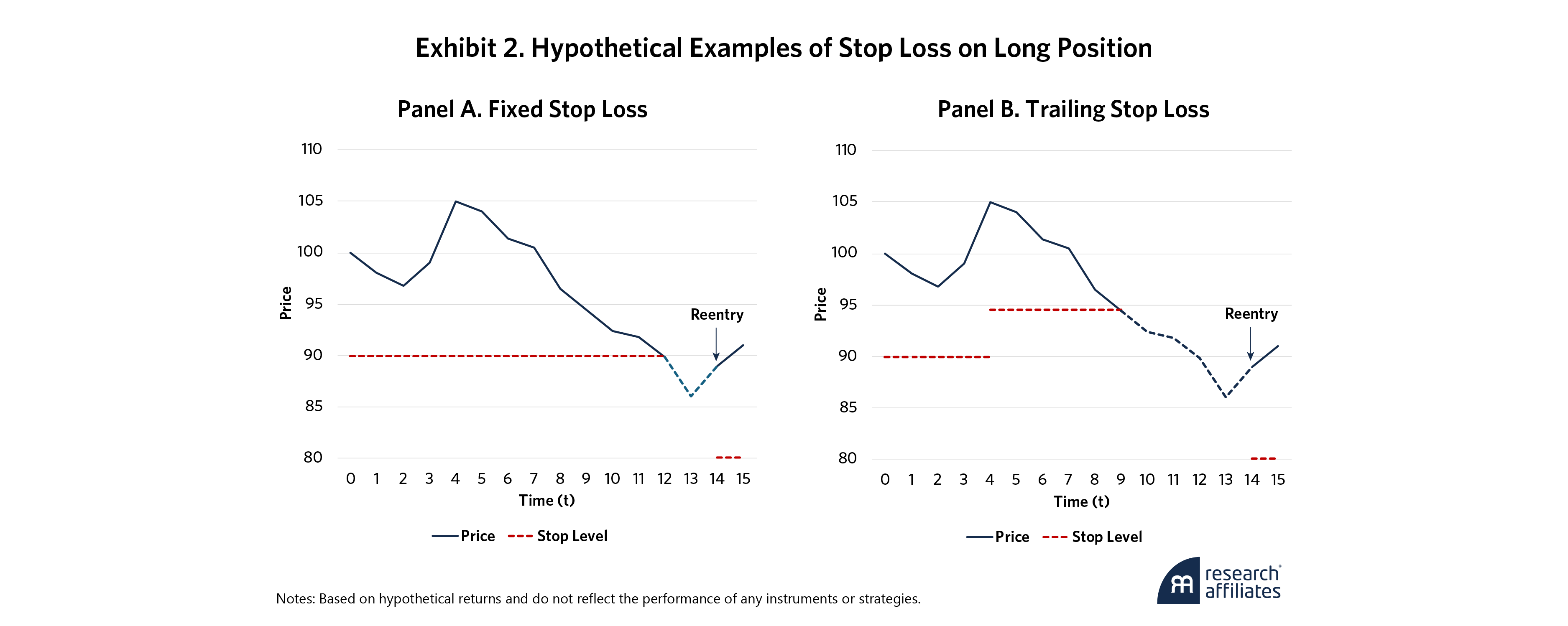
A stop loss is determined by the level at which the position will be closed. For a long position, that is the price at which the investor will sell the instrument. For a short position, it is the reverse. Exhibit 2 shows another important but less-discussed stop-loss parameter: the reentry level. While the stop level reflects the investor’s loss threshold, the reentry level sets the price at which the investor will reopen the position. For long (short) positions this is typically preceded by observation(s) of positive (negative) returns to ensure the position is moving in the desired direction.

There are two types of stop loss: A fixed stop loss is just that – fixed – the stop price is set at an absolute, unchanging value; a trailing stop loss, by contrast, is continuously updated relative to the instrument’s current price (e.g., a 10% loss). The appeal of the trailing stop loss is that it “locks in” some gains when the price of the instrument rises in the case of a long position. Here, we only consider the more preferable trailing stop loss.

“There are two types of stop loss: A fixed stop loss is just that – fixed – the stop price is set at an absolute, unchanging value; a trailing stop loss, by contrast, is continuously updated relative to the instrument’s current price.”

While our approach may sound specific to trading individual instruments, the same principle applies to risk managing baskets of securities. We use stop losses on both individual instrument positions and individual quantitative strategies, or baskets of securities, within an alternative risk premia strategy. Our methodology, however, is generalized for both cases.

Of course, we are not the first to explore stop losses as a portfolio management tool. Our work is heavily motivated by, among others, Acar and Toffel (2000), who apply stop losses to S&P 500, T-bond, and Japanese Yen futures contracts, present stop loss as a risk framework, and identify the conditions under which deploying it may improve performance; Lei and Li (2009), who explore how both fixed and trailing stop-loss rules work on stocks and find the latter performs better as a risk reduction tool; Kaminski and Lo (2014) and Lo and Remorov (2017), who demonstrate that stop loss effectiveness depends on the return-generating process and identify the conditions most associated with successful stop losses; and Arratia and Dorador (2019), who extend these insights by including overnight gaps in the return distributions and show that stop losses can help reduce negative returns.

When Do Stop Losses Work, and When Do They Hurt?

Although exiting a failing position may sound rational, the exit may occur right before the rebound and thus lock in maximum losses. That is why we must first detail the conditions under which stop losses work.

In their seminal paper, Kaminski and Lo (2014) describe the environments in which stop losses mitigate and lock in losses. Specifically, they highlight how stop losses can influence a strategy’s expected returns (“stopping premium”) based on the assumptions underlying the asset’s returns (i.e., return-generating processes). Exhibit 3 shows the various processes and the associated “stopping premium.”

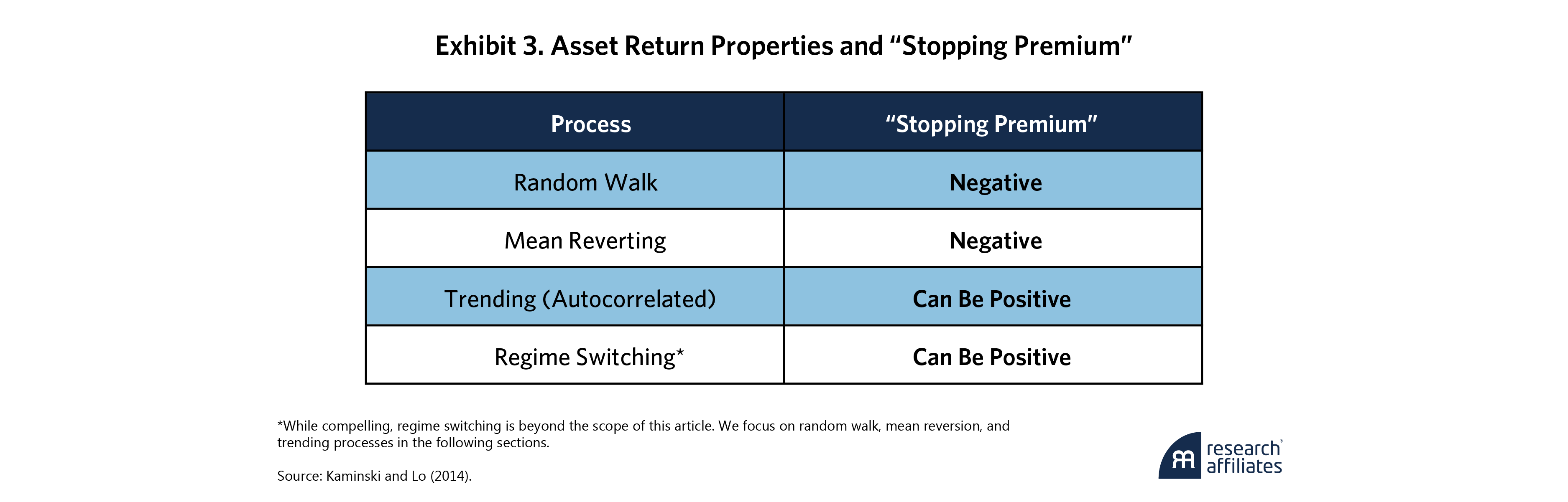
Their findings are intuitive. When a strategy’s returns are unpredictable – a random walk – stop losses should lower returns relative to holding the position, particularly after including transaction costs, because the asset’s next move may or may not be in the investor’s favor. For a mean-reverting process, stopping out of a position often leads to missing the subsequent reversion. However, for trending returns, depending on how autocorrelated they are, the “stopping premium” can be positive as positions moving against the investor will likely continue in that direction. Kaminski and Lo elegantly describe the circumstances when stop losses can be additive:

An autoregressive (AR) model compares the relationship between today’s returns and returns at some point in the past.² In an AR1 model, we measure today’s return against yesterday’s return, and both the magnitude and sign of the AR1 coefficient, Φ, determine the strength of that dependency. Positive values imply persistent returns (e.g., trend). That is, if yesterday’s return was positive, today’s return will likely be positive and vice versa. Negative coefficients imply the opposite. In a mean-reverting process, today’s return will likely move in the opposite direction of yesterday’s return. Finally, of course, an Φ of zero indicates there is no relationship.

Inequality (1) shows that the AR1 coefficient, Φ, must be greater than or equal to the strategy’s Sharpe ratio for stop losses to add value. This is an important connection: It means the consistency in the path of returns must be the driver of the Sharpe ratio for stop losses to be beneficial. That may sound like a high hurdle, but the Sharpe ratio here has to be calculated using the same frequency as the coefficient, Φ. For example, if the AR1 process is estimated with daily returns, an annualized Sharpe ratio threshold of 1.0 would be equivalent to just 0.063 in daily frequency, not such a high hurdle once put in those terms.³

To better illustrate Kaminski and Lo’s findings, we simulate 25-year autoregressive return paths of 100 strategies for each Φ in a range of nine values, from –0.075 to 0.125 in 0.025 increments. We calibrate these 900 simulated strategies to exhibit a daily Sharpe ratio of 0.025 (0.4 annualized) and approximately 15% annualized volatility and apply a 5% stop level and a 0.5% reentry level.⁴

Since we are concerned with the impact of the stop losses, our focus is how the buy-and-hold and the stop-loss applied strategies diverge. To aggregate, we average the differences across the 100 simulations for each Φ. Exhibit 4 shows our results.

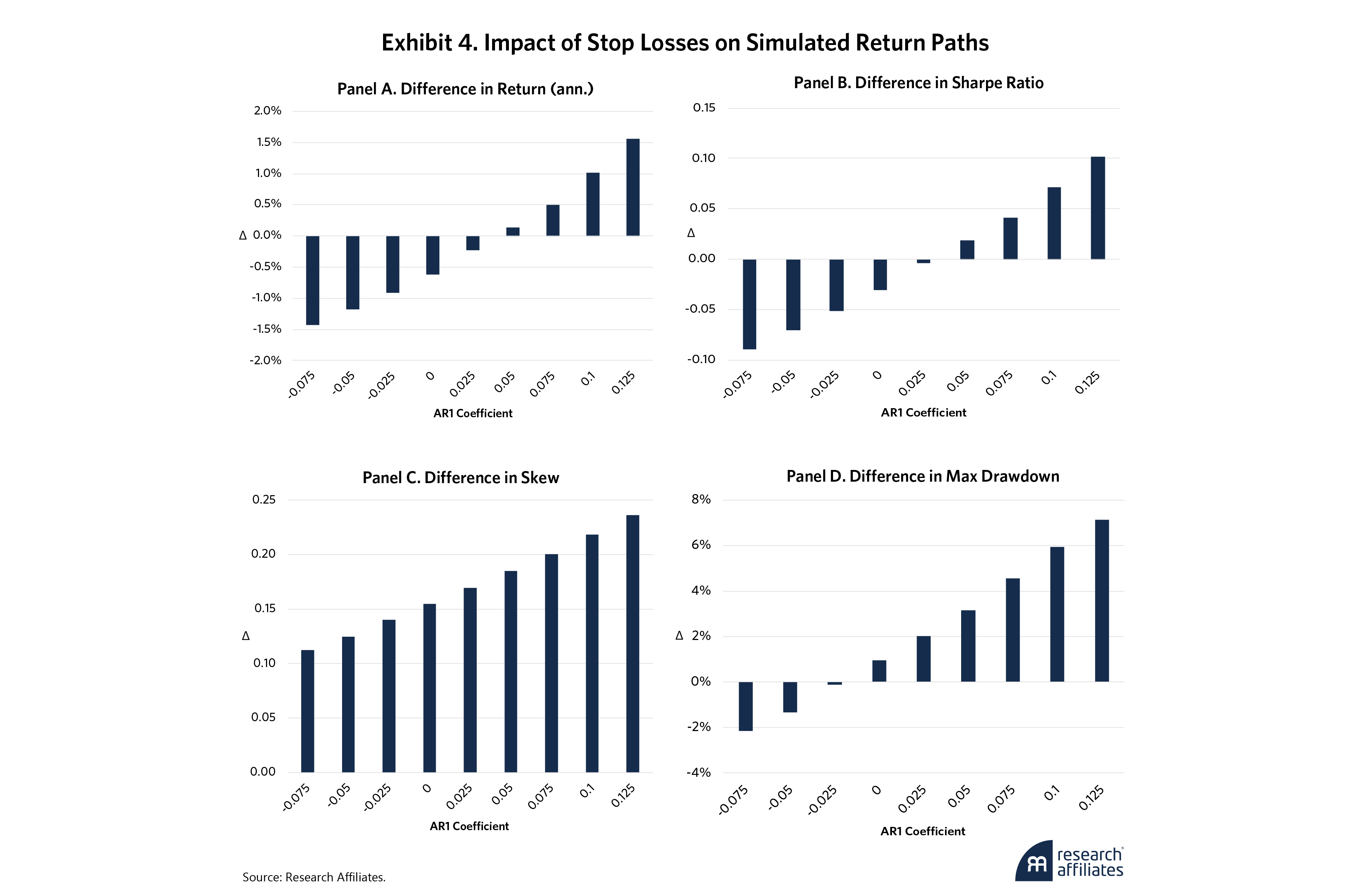
The return and Sharpe ratio differences in Panel A and Panel B are consistent with Kaminski and Lo’s findings. When the AR1 coefficient is exactly equal to the ex-ante Sharpe ratio (0.025) of the simulations, the variations in the returns and Sharpe ratios of the original and the stop-loss-applied strategy are negligible. As the AR1 coefficient increases (decreases) from 0.025, the difference in Sharpe ratio increases (decreases) monotonically.

The risk benefits, on the other hand, are more intriguing. Skewness improves for all values of Φ (Panel B). This implies that stop losses shift the return distribution by reducing either the size or frequency of left tail events, an attractive outcome given the risk-management application that motivated our stop-loss framework. Maximum drawdown differences (Panel C) also suggest that stop losses may even have benefits at Φ = 0 (random walk), which is encouraging if we take the conservative view that the strategy’s returns are completely unpredictable.

Applying Stop Losses to Systematic Strategies

Having confirmed the theoretical results with simulations, we next examine whether stop losses offer similar advantages using real-world systematic strategies. There are many systematic strategies to choose from, but our focus here is ARP and trend-following strategies, which we discuss in Jeon and Masturzo (2024) and Masturzo (2025). Given our interest in stop losses, we build these strategies with relatively simple signals and portfolio construction methods.

The universe for both strategies is identical, encompassing 15 developed market equity index futures; 14 developed market bond futures covering a range of bond tenors; 27 commodity futures, including such sectors as energy, softs, grains, livestock, industrial, and precious metals; and 15 forward contracts of both developed and emerging market currencies against the U.S. dollar.⁵ Rebalancing for each strategy occurs at the end of every month, but stop losses are applied daily, at end-of-day pricing.

Trading-related market frictions are a critical consideration in these backtest exercises. Without modeling for them, we cannot make fully informed investment inferences, especially as they relate to risk-management overlays that introduce additional trading complexities. With this in mind, we include two such frictions in the stop-loss simulations of our two systematic strategies:

• Transactions Cost: For futures contracts, we apply a one-way cost of two ticks per transaction, including the rolling of the contracts. For currency forwards, we assume a 2- and 5-basis-point one-way cost, respectively, for developed (G10) and emerging market currencies.
• Time to Trade: While we calculate desired rebalance and stop-loss trades at end of day, when following instrument-specific trading calendars, transactions are executed at the next day's close.⁶

The results that follow are net of these frictions to provide a better apples-to-apples comparison among the various configurations.

Application 1: Alternative Risk Premia (ARP)

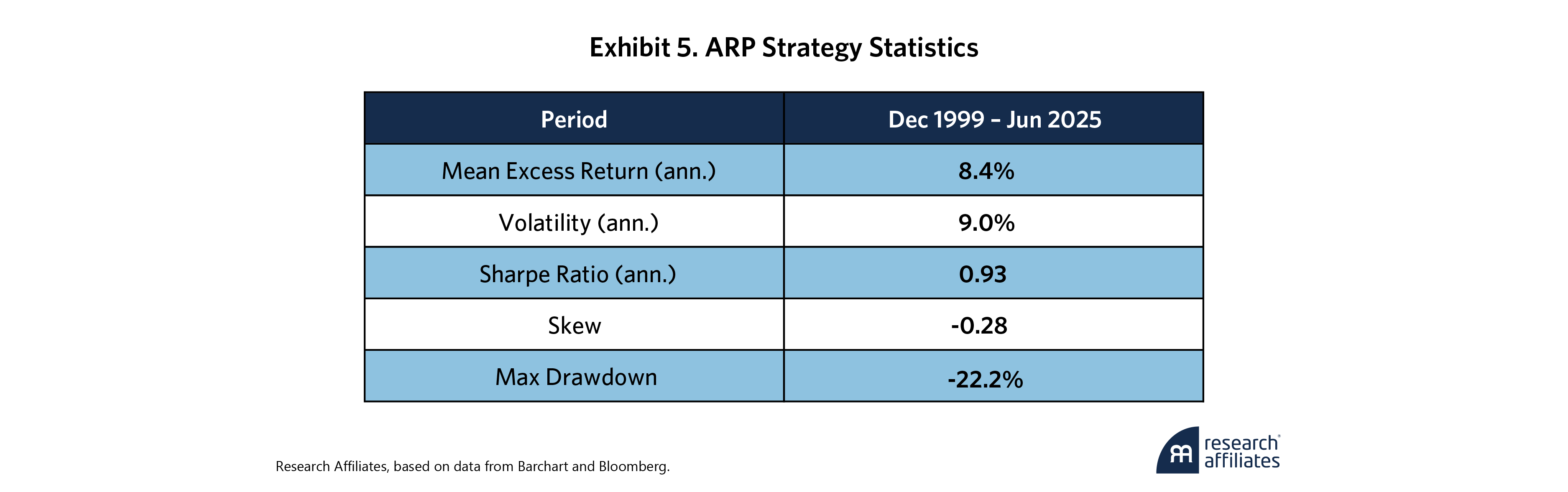
We first generate carry, value, and skew signals across the equity, bond, commodity, and currency asset classes to construct 12 sub-portfolios or sleeves.⁷ To build each sleeve, we first rank the instruments by the signal and then take the top and bottom tertile instruments to form the long and short legs, respectively. Each long or short leg is equal-volatility weighted and sized to be risk-factor neutral in combination. The 12 sleeves are equal-volatility weighted based on a rolling 252-day covariance matrix. Exhibit 5 shows the summary statistics of the strategy over a 25-year backtest period.

Next, we apply stop losses to the ARP strategy at the sleeve-level (e.g., equity carry, bond value) to essentially de-risk the strategy from sleeves that breach the drawdown (stop) limits. This is reminiscent of how central risk desks at multi-manager, multi-strategy hedge funds and “pod shops” manage risk at the aggregate level: They provide specific risk or drawdown budgets to individual portfolio managers and those who exceed those limits can be liquidated or even fired. In our specific case, we acknowledge that “false positives” can activate stop losses and that completely liquidating a diversifying sleeve with a modest Sharpe ratio can be risky itself, and consequently apply two versions of sleeve liquidation: full (100%) and half (50%).

Lastly, to better understand how stop losses perform at varying thresholds, we span the parameter space:

• Stop Level is determined by a number of standard deviations rule. We apply a multiple – 0.1, 0.2, 0.3, 0.4, 0.5 – to the volatility of the sleeve. The smaller the multiplier, the tighter the stop loss, as it will be triggered more often.
• Reentry Level is set by a number of standard deviations rule, with multiples of 0, 0.01, 0.02, 0.03, 0.04, 0.05.⁸ The smaller the multiplier, the lower the requirement to reinvest in the sleeve. For example, a 0 multiplier is equivalent to reentry upon any positive return observation.

Exhibit 6 shows how the original ARP strategy and the stop-loss applied versions compare based on different stop and reentry parameters.

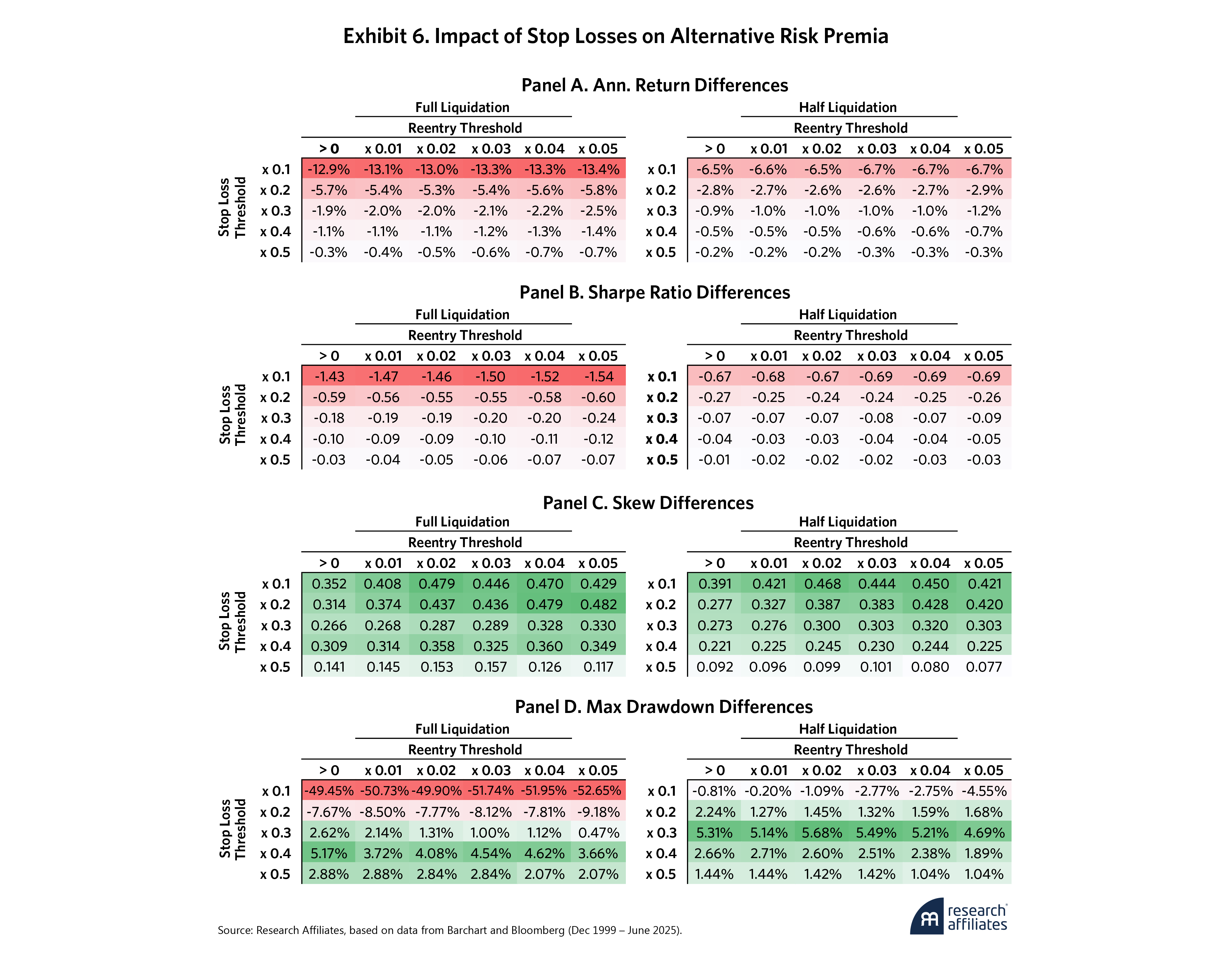
The results are in line with our simulated return paths. No stop-loss parameter improves the returns or Sharpe ratios on a net-of-cost basis (Panel A and Panel B). At extremely tight stop losses (e.g., x0.1), excessive trading creates significant trading friction such that at full liquidation/reentry, the results are strategies with negative Sharpe ratios (recall Exhibit 5’s original Sharpe ratio: 0.93). At more modest thresholds (e.g., x0.3 and higher), however, the performance decline becomes minimal, particularly at half liquidation.

While not surprising, these results reinforce an important point. The stopped-out factor sleeves are included in the strategy in the first place due to a positive unconditional expected return. Removing them would increase trading costs and diminish that positive expected return. If investors only cared about maximizing long-run risk-adjusted returns, stop losses would not be necessary. But that is not the case, and many systematic strategies lack rules to address short-term losses. Additionally, while systematic strategies apply various rules to determine positioning, most include some manager overrides since anticipating every scenario is impossible.⁹ This allows for human input during periods of short-term pain. Add loss aversion and other behavioral biases to this, and we have a perfect storm.

The risk improvement results are similar to what we observe in the simulated return paths. Skewness (Panel C) is improved from the original ARP strategy for all stop-loss parameter combinations. Skew improvements intuitively max out at tight stop losses since they minimize the chances of negative returns compounding and decrease as the thresholds increase. Furthermore, stop losses improve the max drawdown metrics (Panel D), particularly when we avoid the excessive trading costs incurred by the tighter stop losses. This indicates that there are levels of stop losses at which the improvement in risk characteristics may be well worth the small cost in risk-adjusted returns.

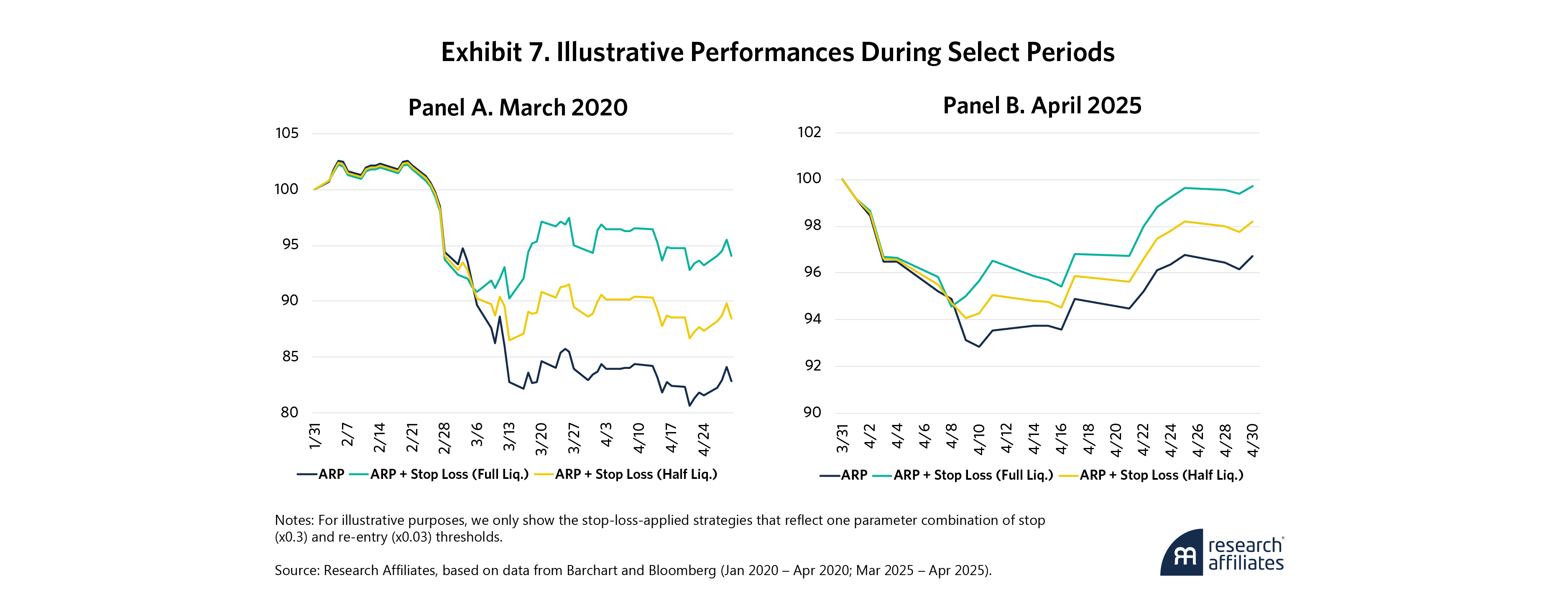
We also examine how stop losses affect the ARP strategy during heightened market uncertainty. Exhibit 7 shows how it weathered the March 2020 COVID-19 crash and the tariff-induced concerns of April 2025. Observing the strategy paths during these times is especially interesting because they indicate how stop losses could reduce emotional reactions (behavioral biases) among managers. Based on the depth of the drawdowns, the stop losses would have added value to the ARP strategy during these periods. By their nature, stop losses make losses inevitable, but their activation may be timely enough, even after accounting for next-day trading, to prevent steeper losses.

Application 2: Trend Following

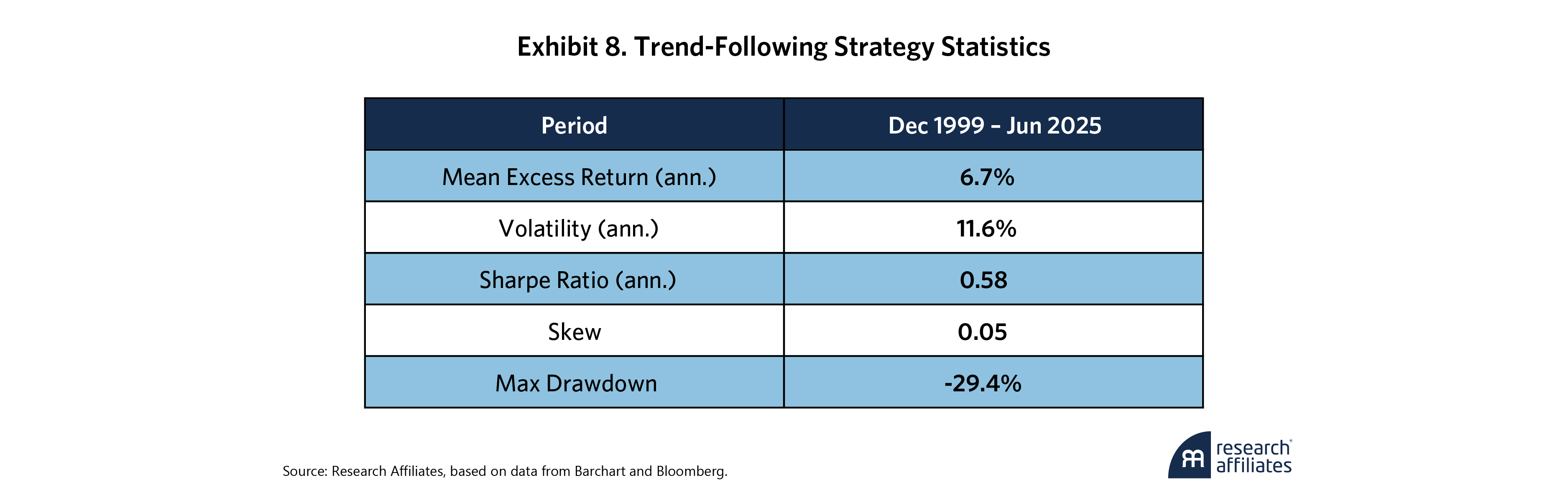
Our trend-following strategy also employs a simple signal and portfolio construction methodology. We apply a one-year (252-day) momentum signal based on which we take directional positions on each of 71 total instruments. All positions are equal-volatility weighted at 10%. Exhibit 8 shows the summary results.

We apply the same stop-loss rules and parameters as in our ARP strategy, except, of course, we implement the stop losses at the instrument level for the trend-following strategy. This makes intuitive sense as the trend-following strategy is essentially making directional bets for each instrument, and we want to limit the losses of those bets. We again sweep across a range of stop and reentry thresholds that we now base on multiples of each instrument’s volatility. Exhibit 9 shows how the stop losses affect the trend-following strategy’s return and risk characteristics.

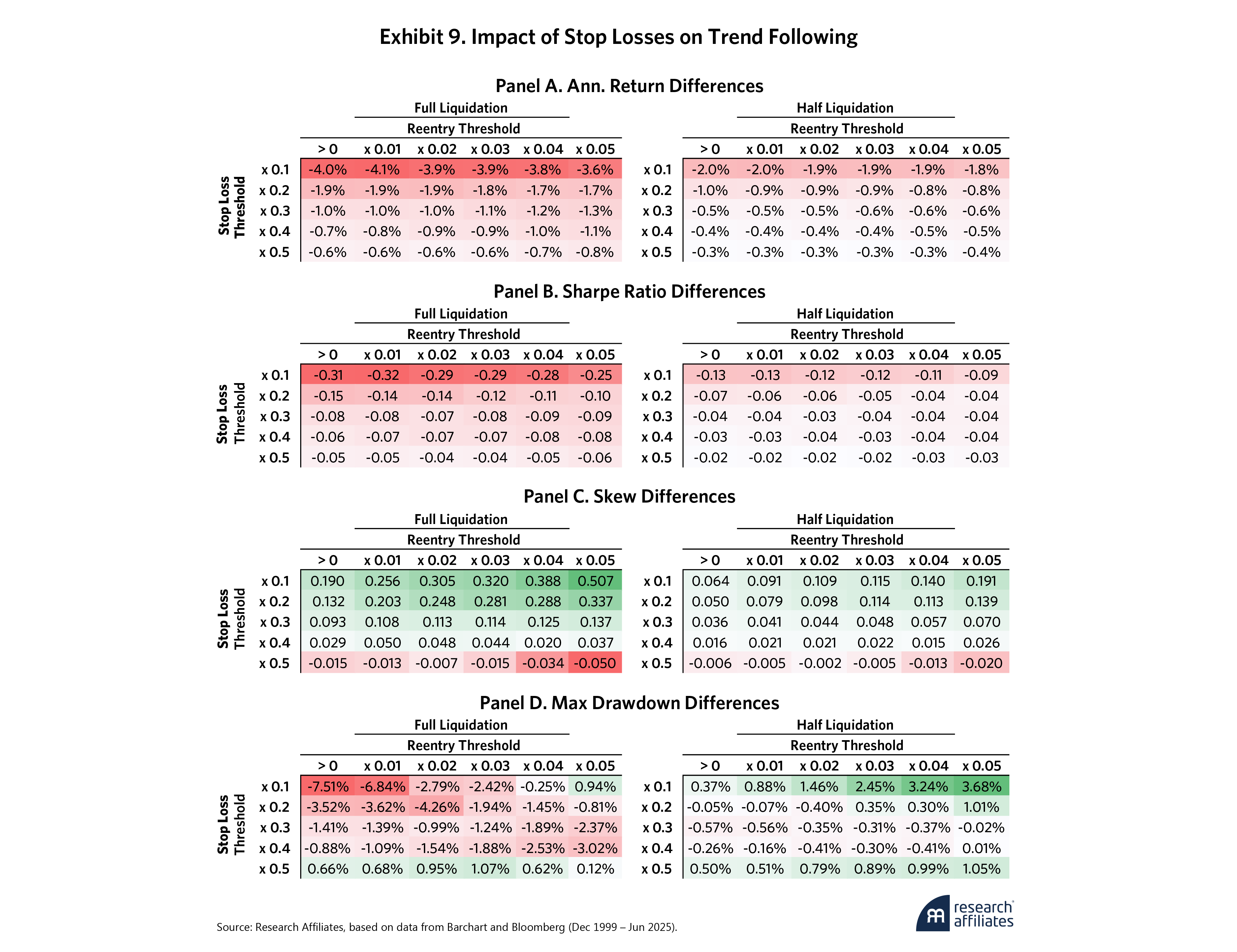
These results generally follow our previous observations on the ARP strategy. A small sacrifice of risk-adjusted returns leads to improved risk characteristics. In the trend-following strategy, implementing a tighter stop loss on each instrument is much less costly than in the ARP strategy. This is likely because applying the stop losses on many individual instruments, instead of just a few strategies as in ARP, diversifies the impact of each stop-loss occurrence. At half liquidation of instrument positions, we can adopt a tight stop loss – 0.2 multiplier – without giving up meaningful levels of Sharpe ratio.

Again, our analysis indicates stop losses improve the skewness of the trend-following strategy, especially at tighter stop losses, though the advantage appears to taper off at wider stop levels (e.g., x0.5). In maximum drawdowns, the trend is less robust. This could be due to myriad effects. For example, the return paths of individual assets can be highly dynamic and mean revert at times, and asset prices may plunge only to rebound sharply within days. Stop losses would certainly underperform in those conditions.

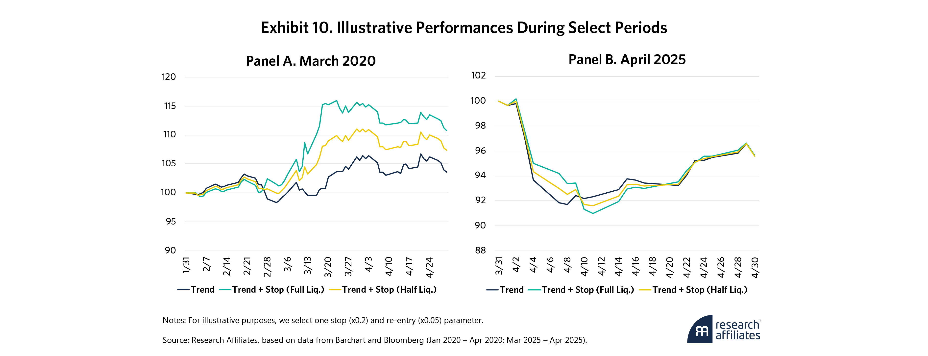
Exhibit 10 reiterates that stop losses are imperfect tools. While stop losses would have added value to a trend-following strategy during the COVID-19 market turbulence (Panel A), they would have been net-even during the April 2025 drawdown (Panel B), particularly after missing the significant post-“Liberation Day” upswing as the combative trade rhetoric subsided. These findings are a good reminder that stop losses may not benefit all strategies all the time.

Finally, it is important to note that in our exercise, we always calculate stop losses at the market close. This could differ from brokerage-implemented stops, which may trigger intra-day and potentially at worse pricing than at end-of-day. While our results are encouraging, real market implementation of stop losses, on single instruments, in particular, requires thoughtful design to avoid these pitfalls.

Conclusion

Stop losses are simple but effective risk tools for managing both systematic and non-rules-based portfolios. Our application of systematic alternative risk premia and trend-following strategies exemplifies this. Our analysis shows that while stop losses rarely enhance expected or risk-adjusted returns, they consistently improve skewness and drawdowns. In certain environments, during market crises for example, stop losses can curb behavioral overreactions and limit catastrophic losses, thereby offering valuable protection even if some performance drag is inevitable.

“Our analysis shows that while stop losses rarely enhance expected or risk-adjusted returns, they consistently improve skewness and drawdowns. In certain environments, during market crises, for example, stop losses can curb behavioral overreactions and limit catastrophic losses.”

For ARP strategies, the risk profile improvement and severe drawdown mitigation may justify modest implementation, especially when trading frictions and diversification from risk premia signals are accounted for. For trend-following strategies, the benefits may be more conditional and depend on the trending nature of the underlying assets. In both cases, stop losses may be value-additive during the worst of times.

Please read our disclosures concurrent with this publication: https://www.researchaffiliates.com/legal/disclosures#investment-adviser-disclosure-and-disclaimers.