Factor Timing: Keep It Simple

by Michael Aked, Research Affiliates

Key Points

• We analyze three factor-timing strategies and find that a strategy based on a factor’s discount (or valuation) and momentum is the most effective tool for determining how to vary a factor’s exposure through time.
• We find that the economic stage six months ahead influences factor returns. Accurately predicting what that stage will be is difficult, however, given current economic forecasting tools.
• Until economic-prediction models can be improved, we find that information gained by estimating the economic stages is already incorporated in a factor’s discount and momentum.

Readers of “Factor Returns’ Relationship with the Economy? It’s Complicated” (Aked, 2020) learned that some degree of variability in a factor’s return across the business cycle exists. Therefore, the ability to add additional sources of return by adding exposure to more than one factor should be of great interest to investors who seek more consistency in shorter-term results.¹ Here, I extend the research of Aked (2020) to help investors better understand how they can vary their factor exposures through factor timing to potentially gain more profitable and more dependable investment results.

Factor timing is the ability to add value to an investment strategy by altering the exposure to various factors through time. I evaluate three factor-timing strategies using 1) a factor’s historical return, 2) the economic stage, and 3) a factor’s discount and momentum. In each case, the strategy is constructed out of sample, using data only available at the time of the specific sample period.

We find that the third strategy, employing a factor’s discount and momentum, is the most effective tool for determining how to vary a factor’s exposure through time. Although a factor’s return changes throughout the business cycle, the ability to predict economic regimes and alter factor allocations accordingly produces less successful results despite being intuitively pleasing. We find that the first strategy, using a factor’s historical performance as a guide to the future, is nearly worthless. Therefore, whereas keeping track of the economy is an important part of the overall investment process, the most important element in factor investing strategies is maintaining a close link to a factor’s discount and momentum.

Factor Portfolio Construction

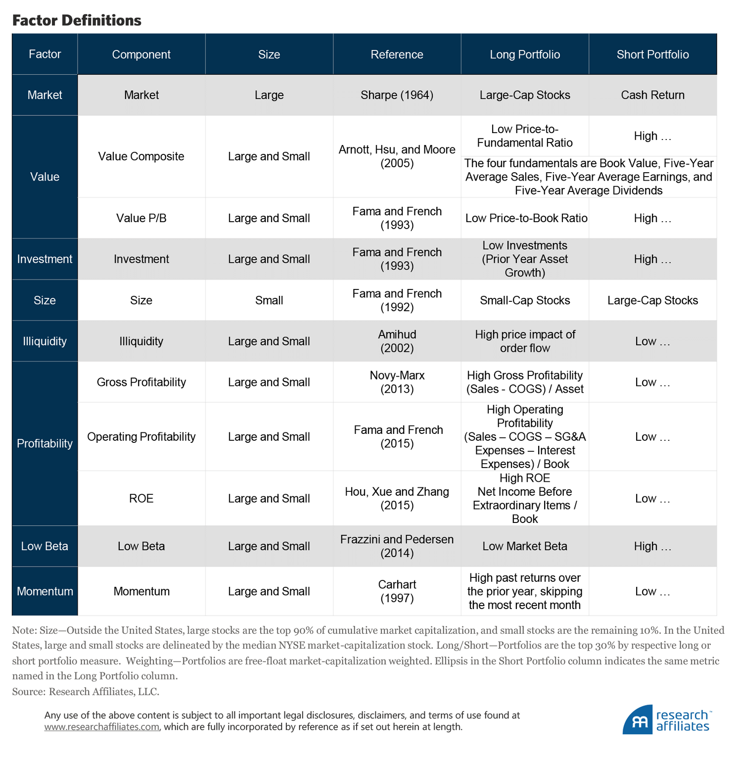
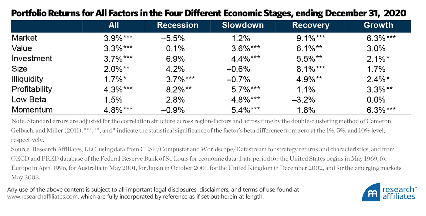
We examine the same eight primary factors as Aked (2020) (market, value, investment, size, illiquidity, profitability, low beta, and momentum) across the same six regions of Australia, United States, Europe, United Kingdom, Japan, and the emerging markets.² Appendix A provides the factor definitions and their returns over the four economic stages.

We construct a small and a large portfolio for each factor, with the exception of market and size. This process yields 14 separate factor portfolios. Because the United States has the longest history, the first month of our analysis period (June 1969) includes only US data. We rank each portfolio by its expected return, and place the highest four in Quartile 4 and the lowest four in Quartile 1, repeating the exercise for the next month, and so on.

We introduce the other five regions into the portfolio construction process as data availability allows. In June 1996, the factor pool widens with the introduction of Europe, increasing the total number of factors to 28 from 14; each factor is constructed in the two regions. At this point, each of the quartiles is composed of 7 factor portfolios. Thus, with four quartiles—a highest-expected-return (Quartile 4) and a lowest-expected-return (Quartile 1) quartile in both regions—we have 28 total region-factors. We continue to progress through time until we reach a total of 70 region-factors, with each quartile containing either 17 or 18 region-factors.

Using Historical Returns for Factor Timing

Some investors assume the historical return of an investment, whether an asset class, an industry, a factor, or an individual equity security, equates with the investment’s future return. This investing approach is the equivalent of driving while looking in the rearview mirror. Nevertheless, because it is a common approach, we consider it as the first potential factor-timing strategy.

We assume the expected return of a region-factor is based on the factor’s historical return. The model calculates the return for the period from the beginning of the dataset through the date at which we build each monthly factor portfolio. The model calculates the historical return across all regions and does not allow a factor’s expected return to vary by region. We only use factor data that were available at the time that we build each month’s factor-timing portfolio.

The model calculates the average annualized return for each of the quartiles. Quartile 1, the lowest-expected-return quartile, has a return of 2.5% a year, and Quartile 4, the highest-expected-return quartile, has a return of 3.8% a year. Each quartile’s return is positive and has a t-statistic well above our threshold of materiality.

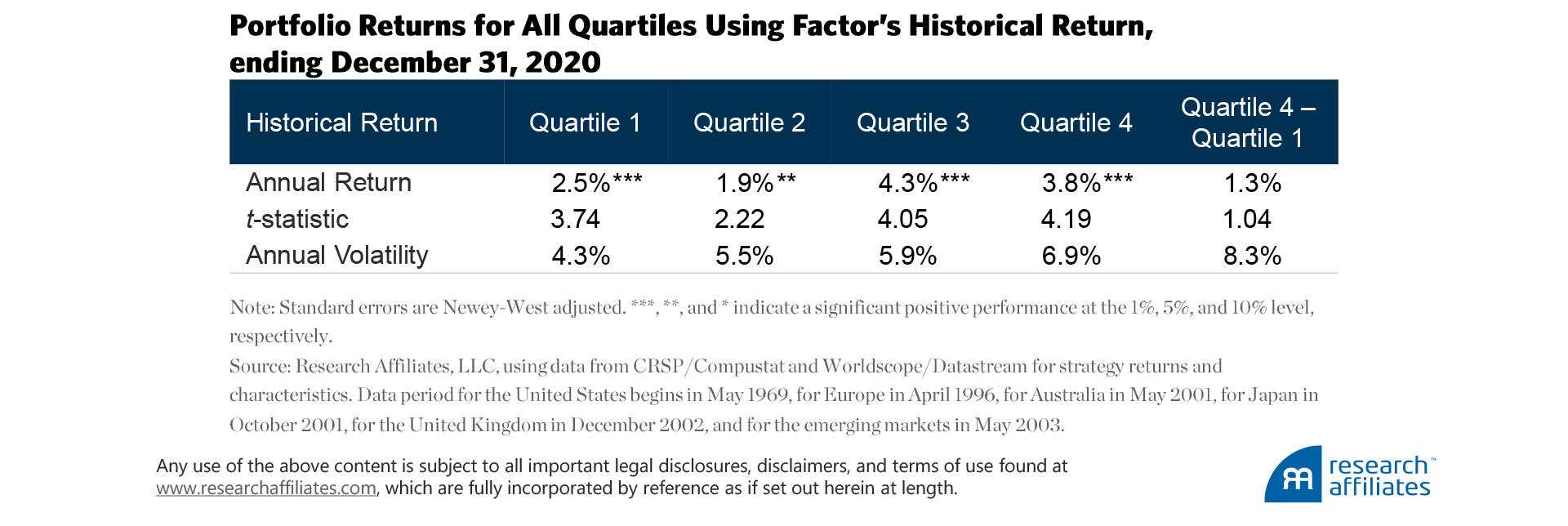
The statistical significance of each quartile’s return should not be a surprise, because the factors we include in our analysis are the best known and most respected by investors in the factor-investing space. The return difference between the top and bottom quartiles, Quartile 4 – Quartile 1, is not significant, however, meaning the annual return difference of 1.3% between these two quartiles can arise from randomness. We thus conclude that factor timing based on the historical returns of well-known factors is not an overly compelling strategy.

Using the Economic Cycle for Factor Timing

We learned, and confirmed our suspicions, that the factors each perform differently across the four stages of the economic cycle (Aked, 2020). The observation alone, however, is not a sufficient condition to profit from this knowledge. To investigate if an investment benefit exists, rather than just an attribution or commentary advantage, we need to generate a quasi-out-of-sample timing strategy³ that employs dynamic factor allocation based on the prediction of economic cycles.

Simply put, the economy matters, and at any point in time, both historically and in the present, information about the economic stage of the world is readily available. Can we profit by applying nowcasting⁴ to forecast a factor’s concurrent and future economic stages in a way that is useful in a factor-timing approach?

For this analysis, we build the factor-timing strategy as described in the previous section, but alter the way we calculate the expected return. Performance of a region-factor takes account of the economic stage. Aked (2020) uses this same analysis. The result is four expected returns, one for each economic stage (recession, slowdown, recovery, and growth) for each of the factors. The next step is estimating the probability of the region-factor being in each economic stage for each month in the sample period.⁵

Because economic data and reporting lag real time (e.g., GDP growth numbers are not reported until after each quarter’s end), our model estimates a factor’s “current” economic stage over its history using nowcasting. In order to predict the upcoming economic stages, our model forecasts economic-stage probabilities 6 and 12 months into the future. Not surprisingly, the further we look into the future, the hazier our view gets. Now, instead of driving while looking in the rearview mirror, at least we are looking out the windscreen, but we can only see so far through the fog.

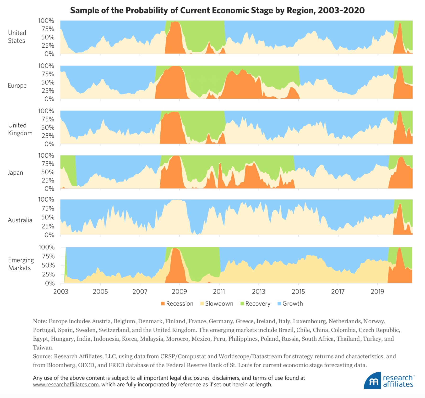For each month, for each region, the model makes a prediction, based only on the data and experience of the economy and the factor up to that point in time. The model estimates the probability of being in each economic stage, then weights the factor’s expected return for each economic stage by the probability associated with that stage. Each region can, and usually does, experience a different economic stage from the other regions. While the global economic environment rhymes across all regions, variability is present in the economic-stage probabilities of the regions.

We repeat our factor-timing strategy, using the economically weighted expected returns of each region-factor. Each month a quarter of the region-factors with the highest expected returns are sorted into Quartile 4, and a quarter of those with the lowest expected returns are sorted into Quartile 1. Of those portfolios classified as being in the concurrent economic cycle, the highest-expected-return quartile, Quartile 4, has an average return of 3.4% a year and the lowest-expected-return quartile, Quartile 1, has an average return of 2.0% a year. The annual return difference, Quartile 4 – Quartile 1, of 1.4% a year with annualized 8.1% volatility and 1.21 t-statistic indicates that forecasting the concurrent economic cycle is of little extra value. Going long (or buying) factors favored by the concurrent economic environment and shorting (or selling) factors that are disadvantaged in the concurrent economic environment is as good as relying on historical winners and losers.

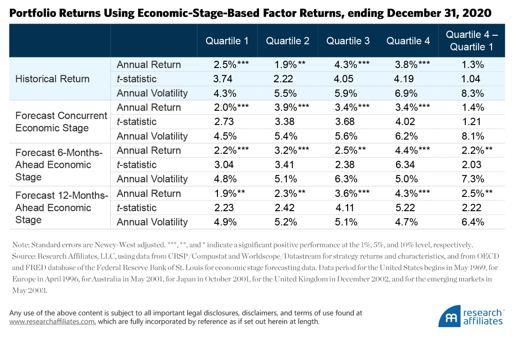
Good evidence exists that the forward economic stage matters far more than the concurrent stage to the performance of factor investing (Aked, 2020). To test this dependency, we forecast the probability of the economic stage 6 and 12 months ahead. Our finding is unsurprising. Building the factor-timing strategy by estimating the economic cycle 6 months out produces a higher, and significantly different to zero, annual return premium (Quartile 4 – Quartile 1) of 2.2% a year. Pushing the economic-stage estimation to 12 months out, the average return difference between highest-expected-return and lowest-expected-return quartiles is even higher at 2.5% a year. Both the 6-month and 12-month forward returns are significantly different from zero.

Using Factor Discount and Momentum for Factor Timing

Incorporating information imparted by the various economic stages being experienced around the world is useful for investors and sure beats relying on factors’ historical returns. That said, successfully using economic-stage forecasting in factor investing is a complicated process. The Research Affiliates investing approach is based on building simple rules-based factor portfolios. Our experience suggests that the less complicated option of using an investment’s discount and momentum—in this case, the region-factor’s discount and moment—can yield better results. A factor portfolio’s discount is calculated as its current valuation (using the relationship of price to various fundamental measures of the component equities) relative to its average historical valuation. A factor’s momentum is the performance of the factor over the previous 12 months.⁶

Over the last few years we have introduced the investment community to the importance of both valuation and momentum, not just as factors in their own right, but drivers of the return to portfolios of assets. Research by Aked, Mazzoleni, and Shakernia (2016) as well as comprehensive research by Arnott et al. (2021) and Ehsani and Linnainmaa (2019) point to momentum having macroeconomic origins. The pattern of returns for momentum indicates a return source driven by the factor exposure of an asset rather than by the idiosyncratic nature of the asset itself. Additionally, Arnott et al. (2019) weigh in on how important valuation is, even at the factor level. Equity factors that are trading at a significant discount (based on fundamental measures such as book value or sales) versus their long-term average valuation produce larger excess returns moving forward than factors’ trading at premiums to their long-term average valuation.

“A factor’s discount and momentum subsumes the investment benefit of our current economic forecasting tools.”

We repeat the same process for building factor-timing portfolios as in the two previous factor-timing strategies. The only difference is that we estimate the future return of a regional strategy based on its own discount and momentum. We do not allow the regions or the factors to respond in a different manner than that dictated by their own discount and momentum. We make this decision because of limited data and because we do not believe the factors would react differently across regions beyond their unique discount and momentum characteristics.

Our results are surprising. Recall that the first factor-timing strategy, which solely considers a factor's historical return, has a quartile spread, Quartile 4 – Quartile 1, of 1.3% a year. We then allow the model’s region-factor return prediction to incorporate the factor portfolio’s discount. In this case, the strategy yields 3.2% a year. If instead, the model’s region-factor return prediction incorporates the factor portfolio’s momentum, the strategy yields 4.1% a year. Finally, if the model allows the region-factor return prediction to incorporate a portfolio’s discount and momentum, the strategy return jumps to 5.5% a year, with a volatility of 9.1% a year, and a t-statistic of 4.83. Discounts and momentum clearly matter! A factor’s discount and momentum are a significant and synergistic determinant of future factor returns.

Recall that the economic forecasting approach to factor timing delivers an average return of 2.2% a year for the 6-month-forward forecasts and 2.5% a year for the 12-month-forward forecasts. An approach that considers either discount or momentum, but not the economic cycle, yields superior returns. And taking into consideration both a factor’s discount and its momentum, again without any economic forecasting, comfortably yields a higher return, with more confidence, at similar volatility. But is that the end of the story? Perhaps combining economic forecasting with a factor’s discount and momentum would lead to even better outcomes and happier investors.

Unfortunately, we find that a factor’s discount and momentum subsumes the investment benefit of our current economic forecasting tools. The reason is not that economic forecasting is not valuable, but that any information we have gained from estimating the economic stages is already incorporated into a factor’s discount and momentum.

“Basing a dynamic factor strategy on a factor’s discount and momentum, investors should be able to generate far more robust outcomes.”

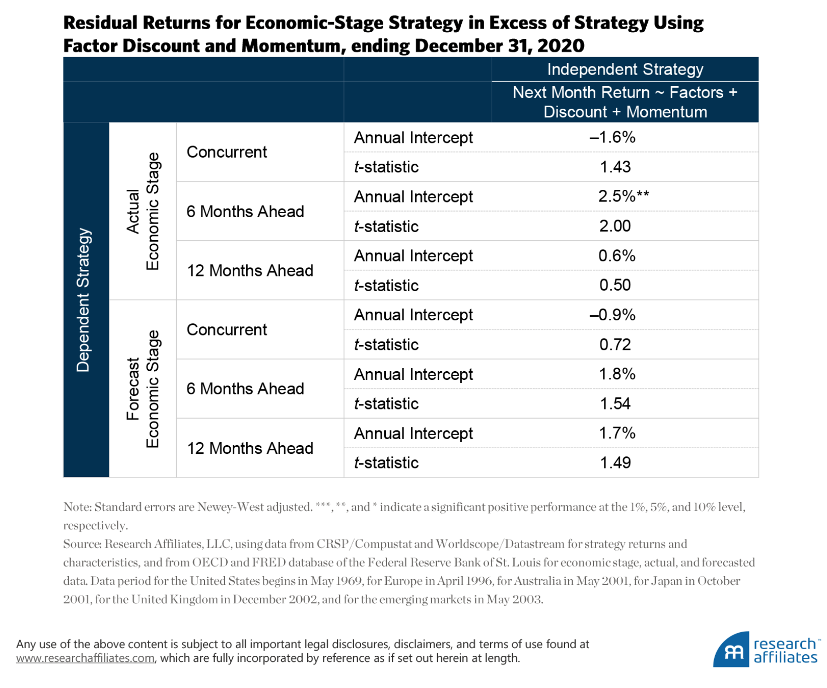
How do we know this? We investigate whether any residual alpha exists from the economic-stage strategies after we account for the impact of a factor’s discount and momentum. Appendix C displays the results from this analysis.

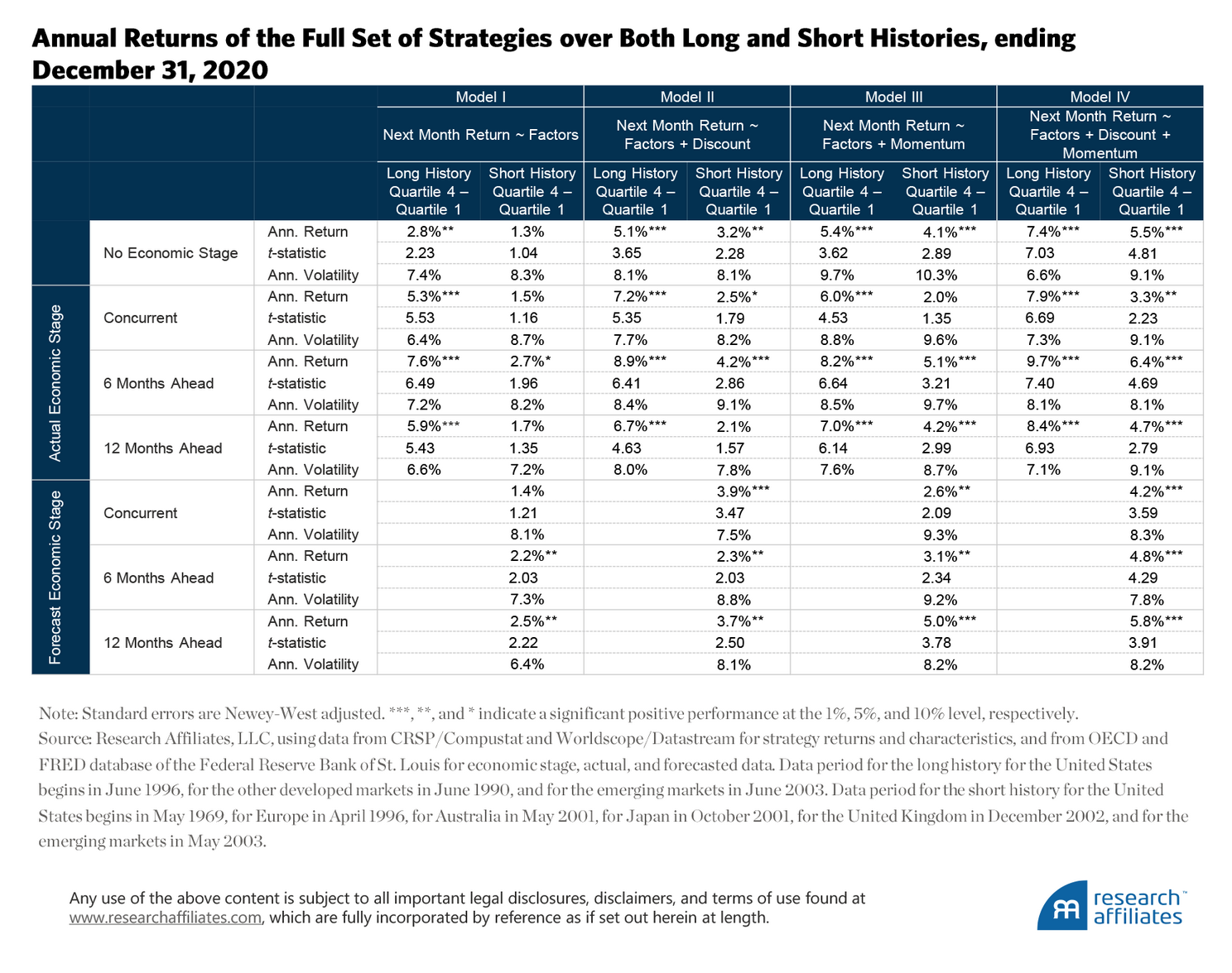
If we use actual economic stages, we find some evidence that knowing the six-month ahead stage would be useful. Unfortunately, such knowledge in the real world is unavailable, forcing us to predict the next economic stage. In this case, the significant 2.5% annualized return from knowing the future falls to an insignificant 1.8% if we must predict the economic stage six months out. Appendix D displays the returns for the full set of strategies.

Next Steps

Having investigated the performance of three factor-timing strategies, we find that just like the market factor, the eight factors we analyze in this article demonstrate an economic-stage preference. Although a differential in performance exists, we show that the momentum and discount, or valuation, of a strategy captures all pertinent information about the current economic cycle.

Thus, although alluring to default to an investment approach based on the economic stage of an economy, it seems to be a siren’s song. By focusing on a much more parsimonious approach of basing a dynamic factor strategy on a factor’s discount and momentum, investors should be able to generate far more robust outcomes.

We also find that the economic stage six months hence influences the factor returns of a market. Undeniably economic prediction is difficult, but continuing to improve economic-prediction models holds value as a means of capturing their influence (even if limited) in a factor-timing strategy. Nonlinear and big data methods may be useful in improving our forecasting ability for regions within the global economy.

Appendix A

Appendix B: Factor-Timing Model

Economic Stage–Based

To determine the economic stages, we collect information on real GDP and the OECD Composite Leading Indicators from the FRED database, with either monthly or quarterly frequency. Additional financial and macroeconomic data for each region are sourced from either the FRED database or Bloomberg. We also calculate the regional factor momentum (the return for the previous 12 months) of the market, value, and momentum portfolios.

We build a hierarchical logit probability regression of the economic stage. First, we estimate the probability of being either in an above- or below-trend growth economic stage. Further, we estimate the probability that, if the economy is growing slower than trend whether the stage is a recession, and if the economy is growing faster than trend whether the stage is a recovery.

In building the quasi-out-of-sample strategy, we take account of the lags in reporting of economic data. We reparameterize the economic-stage prediction model each month using available history at the date of portfolio construction. We lag the use of the economic stage by six months and only use data in the prediction of economic stages if the data were available at the end of the corresponding month-end. For example, January Purchasing Managers’ Index data are released in the first week of February. We therefore lag these data a month so they are first used at the end of February.

Factor Discount and Momentum

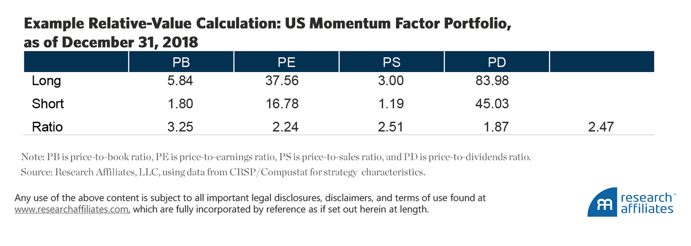
In addition to the monthly performance of each of the 40 factor portfolios, scaled to a 10% a year volatility, we calculate the momentum, last 12-month return, and the discount, which is based on the valuation of the regional factor. The valuation of a regional factor portfolio is the average price ratio of the long portfolio divided by the short portfolio.

We take into account four metrics relative to the market portfolio. For the long and short legs of the factor, we calculate separately the price-to-book (P/B), price-to-equity (P/E), price-to-sales (P/S), and price-to-dividends (P/D) ratios. The long portfolio metric is divided by the short portfolio metric and averaged across all four measures.

For example, the US momentum factor portfolio as of year-end 2018 had a relative valuation of 2.47. We calculate the discount as the full-sample-period regional factor valuation minus the full-sample-period average valuation. A higher discount means the regional factor is cheaper per unit of fundamentals, whereas a lower discount implies the regional factor is more expensive per unit of fundamentals.

Appendix C

Appendix D

Learn More About the Author

Mike Aked, CFADirector of Research for Australia

Endnotes

1. The goal of the new “Your Future, Your Super” proposals from the Australian Treasury Department is to lower the active risk of superannuation investors. The changes will most likely lead superannuation funds to seek more consistent sources of return for their members.
2. Europe includes Austria, Belgium, Denmark, Finland, France, Germany, Greece, Ireland, Italy, Luxembourg, Netherlands, Norway, Portugal, Spain, Sweden, Switzerland, and the United Kingdom. The emerging markets include Brazil, Chile, China, Colombia, Czech Republic, Egypt, Hungary, India, Indonesia, Korea, Malaysia, Morocco, Mexico, Peru, Philippines, Poland, Russia, South Africa, Thailand, Turkey, and Taiwan.
3. Our quasi-out-of-sample strategy parameterizes our models using only the information available at the time. For example, data used in regressions and estimations for, say January 2000, would had to have been available at the end of December 1999. We call it a quasi-out-of-sample strategy because our model and strategy selection has the advantage of being able to choose from historical data as appropriate; only the performance of a factor strategy after the research supporting the new factor has been published can be truly out of sample.
4. The term nowcasting, as defined by Arnott and Treussard (2020), has two meanings. One is the use by economists to estimate an economic measure, such as quarterly GDP growth, based on currently available interim data. The second is the use by pundits, financial media, and market prognosticators to “forecast” the direction of capital markets by applying an explanation of what has happened as an explanation of what will happen. The former is a legitimate use, the latter can be very dangerous.
5. The model we use to estimate the economic stage is in Appendix B. If you are interested in further details, please contact us.
6. Appendix B provides more details on calculating the discount and momentum of a region-factor (or any portfolio for that matter).

References

Aked, Michael. 2020. “Factor Returns’ Relationship with the Economy. It’s Complicated.” Research Affiliates Publications (November).

Aked, Michael, Michele Mazzoleni, and Omid Shakernia. 2016. “When a Storm Is in the Offing: Fundamental Growth in the U.S. Equity Market.” Research Affiliates (June).

Amihud, Yakov. 2002. “Illiquidity and Stock Returns: Cross-Section and Time-Series Effects.” Journal of Financial Markets, vol. 5, no. 1 (January):31–56.

Arnott, Robert D., Mark Clements, Vitali Kalesnik, and Juhani Linnainmaa. 2021. “Factor Momentum.” (March 22). Available at SSRN.

Arnott, Robert D., Campbell R. Harvey, Vitali Kalesnik, and Juhani Linnainmaa. 2019. “Alice’s Adventures in Factorland: Three Blunders That Plague Factor Investing.” Journal of Wealth Management, vol. 45, no. 4 (April):18–36.

Arnott, Robert D., and Jonathan Treussard. 2020. “Forecasts or Nowcasts? What’s on the Horizon for the 2020s?” Research Affiliates Publications (January.)

Cameron Colin, Jonah Gelbach, and Douglas Miller. 2011. “Robust Inference with Multiway Clustering.” Journal of Business & Economic Statistics, vol. 29, no. 2 (January):238–249.

Carhart, Mark M. 1997. “On Persistence in Mutual Fund Performance.” Journal of Finance, vol. 52, no. 1 (March):57–82.

Ehsani, Sina, and Juhani Linnainmaa. 2019. “Factor Momentum and the Momentum Factor.” NBER Working Paper No. w25551. Available at SSRN.

Fama, Eugene F., and Kenneth R. French. 1992. “The Cross-Section of Expected Stock Returns.” Journal of Finance, vol. 47, no. 2 (June):427–465.

———. 1993. “Common Risk Factors in the Returns on Stocks and Bonds.” Journal of Financial Economics, vol. 33, no. 1 (February):3–56.

———. 2015. “A Five-Factor Asset Pricing Model.” Journal of Financial Economics, vol. 116, no. 1 (January):1–22.

Frazzini, Andrea, and Lasse Heje Pedersen. 2014. “Betting Against Beta.” Journal of Financial Economics, vol. 111, no. 1 (January):1–25.

Novy-Marx, Robert. 2013. “The Other Side of Value: The Gross Profitability Premium.” Journal of Financial Economics, vol. 108, no. 1 (April):1–28.

Sharpe, William F. 1964. “Capital Asset Prices: A Theory of Market Equilibrium under Conditions of Risk.” Journal of Finance, vol. 19, no. 3 (September):425–442

Copyright © Research Affiliates