Wild, But Not Crazy
by Clifford Asness, Ph. D. AQR Capital Management, Inc.
You don’t need me to tell you that markets have been pretty wild lately. But, perhaps I can help with a little perspective versus history, and try to home in on what was merely big about these past few days versus what was really really big. Warning, this one gets a bit wonky with some number overload.
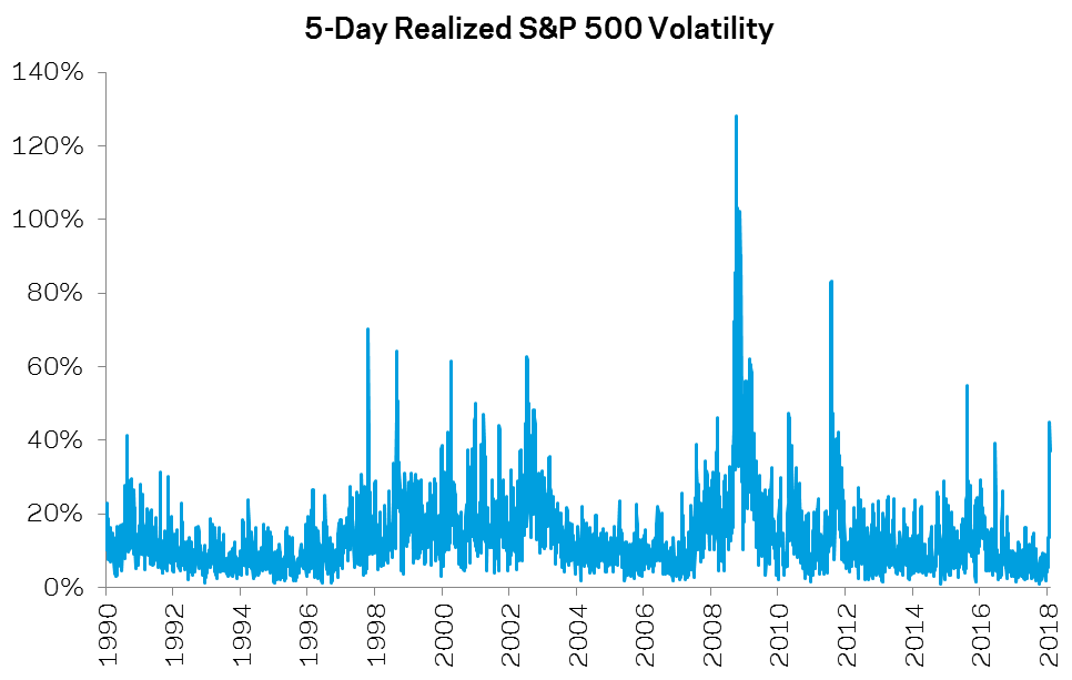
In this note, I look at rolling 5-day daily volatility of the S&P 500 starting from 1990, when we also have data on the VIX.1,2,3 For the five days central to this swoon (2/2/2018 – 2/8/20184) the annualized daily volatility was 38.9%.5,6 That’s big. But we’ve seen much bigger. The maximum occurred, not surprisingly, in the teeth of the Global Financial Crisis (10/09/2008 – 10/15/2008), hitting 128.2% annualized over those five days (and a nice example of the silliness of annualizing 5-day events!). The 99th percentile 5-day rolling volatility from 1990-present is 55.5%, and the recent 5-day period of 38.9% registers a 97th percentile. Sure, those are big outcomes, but two standard deviation events are a dime a dozen in financial markets. To put it into perspective, below I graph this realized 5-day volatility back to 1990.

Source: Bloomberg, AQR, Jan 9, 1990 through Feb 12, 2018. For illustrative purposes only.
Clearly recent events were big, but similar things have occurred quite a few times, and much bigger ones happened during the GFC.
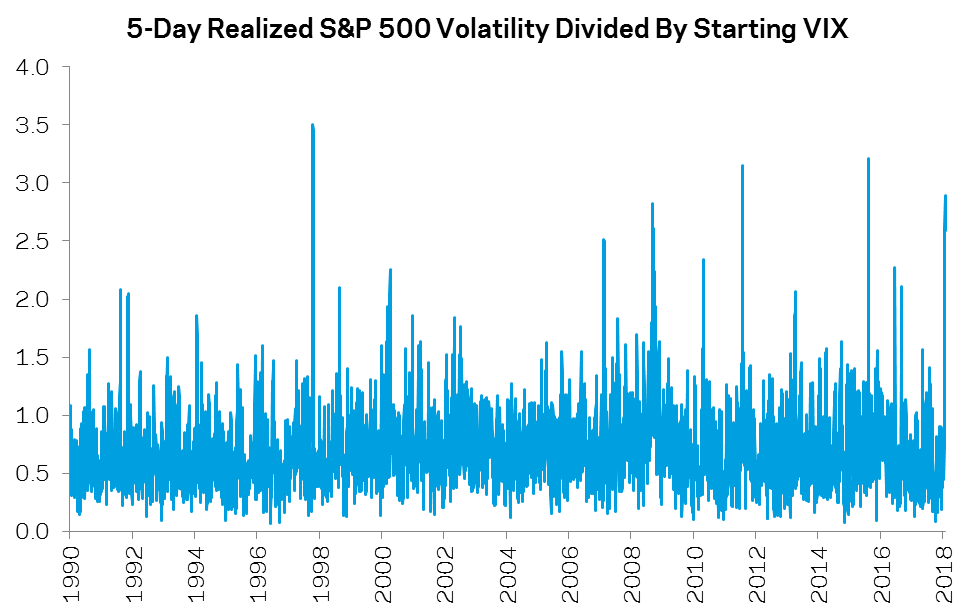
Now, let’s look at it slightly differently. We’re still sticking with our very short-term 5-day volatility measure, but now let’s look at it as a ratio to the level of the VIX at the start of each 5-day period. This is potentially very different. To the extent the VIX measures forward-looking volatility expectations, this ratio is a measure of how surprising, not simply how big, 5-day volatility turned out to be. As the graph below shows, at the worst drawdown during this recent period, 5-day realized volatility (38.9%) was a whopping 2.9x larger than the starting VIX level (13.5%). This was a +3.3 standard deviation event (again, using logs to normalize the series), which is extreme but still something that occasionally happens per the graph below. Clearly, the recent downturn has been more extreme versus the past in terms of “surprise volatility,” as compared to simply volatility itself. In particular, note that the GFC still produces some biggies, but not wildly larger surprises versus other periods as the volatility was less surprising (it didn’t come as much out of the blue as the VIX correctly ex ante captured some of it, likely because trailing volatility was high for a while).

Source: Bloomberg, AQR, Jan 9, 1990 through Feb 12, 2018. For illustrative purposes only.
The maximum ratio ever hit was 3.5x (over the period 10/22/1997 – 10/28/1997), when U.S. stock markets declined during the 1997 Asian financial crisis. This 1997 maximum surprise came about in a somewhat different way than recent events. Unlike last week, the VIX didn’t start this 1997 stretch low and then get hit with big vol. Rather, it began on 10/21/1997 with a VIX of 19.5%, which is the 60th percentile (last week’s drawdown began from a VIX of 13.5% which is the 24th percentile7) and then experienced a 68.4% annualized 5-day volatility (99th percentile), considerably higher than last week’s high levels. The story of 1997’s surprise was extremely high realized volatility (though not hitting 2008 levels, which were even higher, but not a bigger surprise – yes, I know it’s getting a little hairy in here!) compared to an above average starting VIX. In slight contrast, last week’s surprise was quite high, but it came from less extreme realized volatility (a recent level of 38.9% for the 5-day drawdown period and a max of 44.9% shifting to one day later vs. 68.4% in the 1997 event) compared to a fairly low starting VIX. This highlights how looking at surprises can be somewhat different than just looking at volatile periods. The very recent surprise was high, similar to the 1997 surprise, but the absolute level of volatility wasn’t as extraordinary.
Now let’s apply the above to examine a real life investing issue. Some investors use volatility forecasts to vary their investment size in an attempt to target more stable returns, effectively holding larger positions after periods of low volatility (or a low VIX8) and smaller positions after periods of high volatility (with an assumption that volatility is fairly “sticky” so these trailing levels have power to forecast the upcoming future). Recent events have to be pretty bad for those who try to target such a constant volatility, right? They must have been positioned way too aggressively given the VIX was so low, and thus, had to get hit much harder by the surprise in realized volatility, right? Well, in a word, yes. But that’s not the whole story by a long-shot.
To study this, I build a toy risk-model (that is, a risk-model I hope gets at the main point but is way simpler than one you’d likely use in real life). I imagine an investor trying to target a 15%9 constant volatility exposure to the S&P 500 (or, to be fussy, the S&P 500 and cash, as varying the amount of cash is how this is done) using today’s VIX to make the decision whether to lever up (when the VIX is forecasting lower than 15% volatility) or de-lever (when the VIX is forecasting higher than 15% volatility). Now, even in a toy model, I can’t just use a VIX of 25 to say “the VIX is forecasting a 25% annualized volatility.” That toy would be broken at the get-go. The VIX reflects option-based implied volatilities that average decently higher than realized volatility (leading to the so-called volatility or variance risk premium). So I enhance the risk-model (though I’d still call it a toy!) to adjust for the VIX’s average overstatement.I look back over the prior rolling three years and measure the ratio of the median VIX to the median realized 5-day S&P 500 volatility, and use this ratio in conjunction with the VIX level to size positions at each point in time. So if that ratio has been 1.5x (meaning the VIX overstated volatility by 50%) over the last three years and the VIX is at 30 now, I’d use 20% (30 divided by 1.5) for predicted volatility. So, in this case, to keep a constant 15% volatility I’d de-lever the S&P by being 75% long (15%/20%).10,11 Got it?☺
So imagine you used this way-too-simple model to manage your S&P 500 exposure from 1993 - present.12 That is, instead of a regular S&P 500 index fund, you ran a “constant vol” S&P 500 index fund using this method. First, your price return was about 2% better per annum. I don’t take that too seriously. Even 25 years isn’t that long to estimate mean returns (and I know that in some other asset classes, like bonds, this has gone the other way over this period).13 This is about volatility/downside management so that’s what I focus on next.
Well, not surprisingly, the recent swoon was indeed worse for the constant vol crowd. The S&P’s recent drawdown (1/29/2018 – 2/8/2018) was -10.2% while the (toy risk-model) constant vol targeters fell -14.5%. Sounds ugly. And indeed it was ugly, as you’d expect for such a big surprise that starts from a low vol (and thus high exposure for vol targeters) place. If one takes the full series (1993 - present) targeted vol S&P 500 daily return compounded over these nine days and subtracts the regular S&P 500 daily return, the -4.3% difference (-14.5% vs. -10.2%) was a -3.3 standard deviation event.14,15 So, we are definitely looking at a pretty bad event for those targeting volatility. That’s the view from the trees of recent turmoil. Let’s move to the forest.
Let’s look at the risk characteristics over not just the recent turmoil but the whole 1993 - present experience (which certainly includes the recent big moves). The S&P 500’s daily returns over this period realized an annualized volatility of 17.7%16, a skewness of -0.1, and a kurtosis of 9.5 (extremely “non-normal”). The volatility-targeted S&P 500’s daily returns realized an annualized volatility of 16.9%, a skewness of -0.4, and a far more “normal” kurtosis of 1.7. The worst day for the S&P 500 was -9.0% vs. -7.7% for the vol-targeted version.
Over 20-day rolling return windows, the regular S&P 500 delivered a skewness of -0.8 and a kurtosis of 4.1, vs. -0.1 and 0.2 for the very “normal” looking vol-targeted version from 1993 - present. The worst rolling 20-day period was -28.2% for the S&P 500 versus a way smaller -15.1% for the vol-targeted series. Looking at one year rolling return windows, the worst case for the S&P 500 was -49.1% vs. -34.6% for the vol-targeted investment (both series start to look pretty normally distributed at the rolling annual horizon).17 Finally, if we look at the worst drawdowns over the whole sample, the S&P 500 comes in at 56.8% with the vol-targeted version at -48.8% (sorry, vol targeting can’t save you from bad times, though perhaps can sometimes make them a bit less painful).18
The point here isn’t to extoll this exceedingly simple model or even volatility targeting itself. The point is that anything should be evaluated over as long a time-frame as possible (and for which you have relevant data). Over this 25-year period, using just the VIX (adjusted for its average overstatement) to target volatility has led to a decently more stable investment than just the S&P 500 itself, even considering the recent surprise that’s gone against it, and total returns at least as good (recall they were actually considerably better but we, mostly, don’t believe that’s a permanent property of this approach).
Back to our main story. As of now (no predictions going forward!) this recent wild period is not super crazy when we look just at volatility itself (it’s high, but not super high vs. history). But, when we look at it as a surprise (by comparing the realized 5-day volatility to the starting VIX) it’s a considerably more shocking event, though still not unprecedented. Similar events have occurred five or so times in the 1990 - present history (again, see the above figure). Finally, when just using the simple method of targeting constant volatility that we employ here, this recent surprise swoon was, as we’d expect, pretty bad for volatility targeters. But, over the longer term, volatility targeting, even the super simple volatility targeting our toy risk-model employs, may, on average, deliver more downside stability than not volatility targeting and implicitly letting the market dictate the volatility of your investment.
[1] Yeah, with only five data points I know that’s a crazy number, so don’t take this as gospel. If anyone wants to study this more, using lots of different specifications, please send me the results! Another thing to try, which I doubt will change things, but worth looking at, is to use 5-day average squared returns instead of volatility (as volatility subtracts the mean which doesn’t make a ton of sense over five days but is easier for old men to do in Excel). [2] Returns used here are close-to-close differences in logged prices or, put differently, continuously compounded price return. They are a bit better behaved than simple compound returns. Plus, I always feel smarter using logs. [3] Yes, after telling people to stop talking about the VIX so much I’m now talking about it. Results don’t change very much if, instead of using the VIX, I use some relatively short-term measure of realized trailing volatility. [4] My convention here is 2/2/2018 – 2/8/2018 is inclusive of the returns on 2/2 and 2/8. [5] Note that by choosing a 5-day period we already know to be an extreme one, we also know going in that we’re going to see big somewhat “non-normal” looking results, as is common for ex post order statistics. [6] These five days are the drawdown period, but not quite the maximum realized 5-day volatility, which actually came a day later at 44.9%, dropping one of the big losses and adding in a big rebound day (you can see it edging over 40% in the upcoming graph). [7] And it had already risen from its YTD low of 9.1%. [8] Recall again these are nearly the same thing. [9] If instead of this somewhat arbitrary 15% we used a trailing long window to estimate realized S&P 500 volatility and then target that going forward, we find very similar results. It’s just that 15% is much easier to explain! [10] For all of this I only use the S&P 500 price, not total return. If that matters for this exercise I’ll be quite surprised, but friendly readers can check this for me! [11] This ratio was indeed 1.4x (median) and 1.5x (mean) from 1993 - present. [12] The VIX starts in 1990 and we need three years of data for our look-back. [13] In fact, I may be too dismissive here. The long-run return edge of vol-targeted strategies is not merely something we observe in data with no explanation; there is also a potential logic behind it. If, as many have pointed out, high volatility periods often coincide with bear markets, you are taking smaller positions when the market has done poorly recently and vice versa. That is, this process likely entails at least some exposure to trend-following (albeit perhaps to shorter-term trend following than we usually study) and there’s lots of evidence that this has some efficacy (of course, this is not the most direct way to measure trends). Also, while trading costs, using say S&P 500 index futures, may be low, they will, of course, reduce the returns of real-life volatility targeters. [14] Again, keep in mind that standard deviation events when you ex post choose a precisely terrible period (as we’ve done here choosing these exact nine days) will tend to be large. To further put it into perspective, the biggest 9-day victory for volatility targeting over the standard S&P was +13.0% while the biggest 9-day loss was -11.9% over this period. [15] One of the many things not explored in constructing this “toy risk-model” approach is using leverage caps (or, equivalently, systematically not believing a volatility reading below some pre-specified level). We believe this is quite common among those employing this type process and we’d recommend it. It has the potential to reduce some of the larger differences between targeting and the standard approaches and any “non-toy risk model” should consider them. [16] Note our toy model was trying to target 15.0% and delivered 16.9%. That’s mostly because you never get precisely your point estimate, and likely somewhat because this toy model is just a toy. [17] We are far from the first to note that things tend to look much more “normal” at all but relatively short time horizons. For an excellent example studying the GFC look here. [18] Remember, I’m just looking at price returns so the model drawdowns here will be a bit worse than those actually experienced by investors who, of course, receive dividends.This post was originally published at AQR Capital
Copyright © AQR Capital


