by Jim Masturzo, Senior Vice President, Asset Allocation, Research Affiliates
Key Points
- The one-factor CAPE model better predicted market returns than a simple yield-plus-growth model in five straight decades, before underperforming in three of the last four.
- Although CAPE is often intimated as a one-size-fits-all tool, no single model is a silver bullet applicable to all markets, all the time.
- The Research Affiliates new Asset Allocation Interactive platform offers multiple expected return models, which can be blended together to create optimal portfolios containing the best of each model’s perspective.
For close to three years, Research Affiliates has been publically providing long-term expected returns across a variety of asset classes with our Asset Allocation Interactive platform (AAI platform), available on our website. The feedback from the investment community has been overwhelmingly supportive. So supportive, in fact, that we decided to overhaul the original website to add more data and functionality. Still free of charge, we are excited to roll out in June 2017 our newly enhanced website offering even more analytics for asset allocators.
I admit it—I’m suffering from fatigue related to the cyclically adjusted price-to-earnings (P/E) ratio (CAPE), which—for the unfamiliar—measures the ratio of price to an average of real earnings per share over the previous 10 years. As you can imagine, having CAPE fatigue at Research Affiliates makes me as popular as Ronald Miller at the end of the cult 1987 classic Can’t Buy Me Love—I’m eating lunch alone.
Nevertheless, basing expectations on CAPE is certainly not the worst thing an investor can do. We believe that distinction is most appropriately awarded to the commonly used historical-average model that simply extrapolates historical returns into future expectations. Some investors, however, have graduated from the historical-average model to following the advice of practitioners who espouse the wonders of the CAPE ratio—all the time, and forever.
CAPE fatigue is less an incrimination of CAPE as it is of the “one model all the time” approach. Instead of focusing completely on one framework for estimating future returns, investors benefit from considering multiple perspectives—the approach we take in our AAI platform. In this article, we look at three different models of return estimation along with the benefits for investors of incorporating multiple expected return models in their investment strategy.
Birth of CAPE
Campbell and Shiller (1988) is the genesis of CAPE’s rise in popularity. The backstory of the CAPE ratio, more colloquially known as the Shiller P/E ratio, is its usefulness in identifying if the market is under-, fairly, or overvalued because of the significant relationship between the current level of the ratio and the real total return of the market over the subsequent decade. Campbell and Shiller demonstrated this relationship in the US equity market for the period 1881 to 1987.
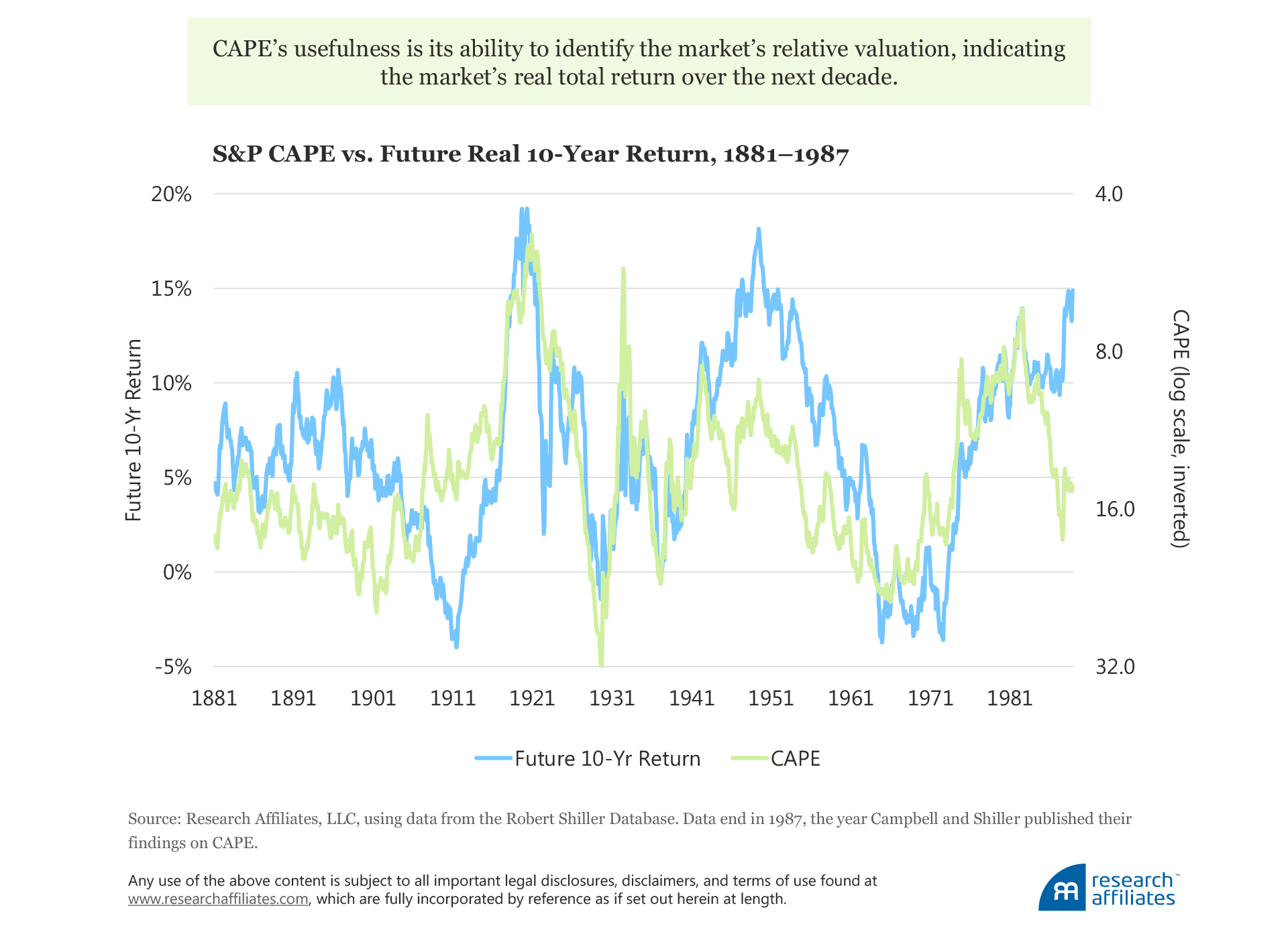
If we regress the inflation-adjusted future real 10-year returns on the CAPE ratio, we get the following equation:1
Returnt,t+10 = –9% × ln(CAPEt) + 31.1%
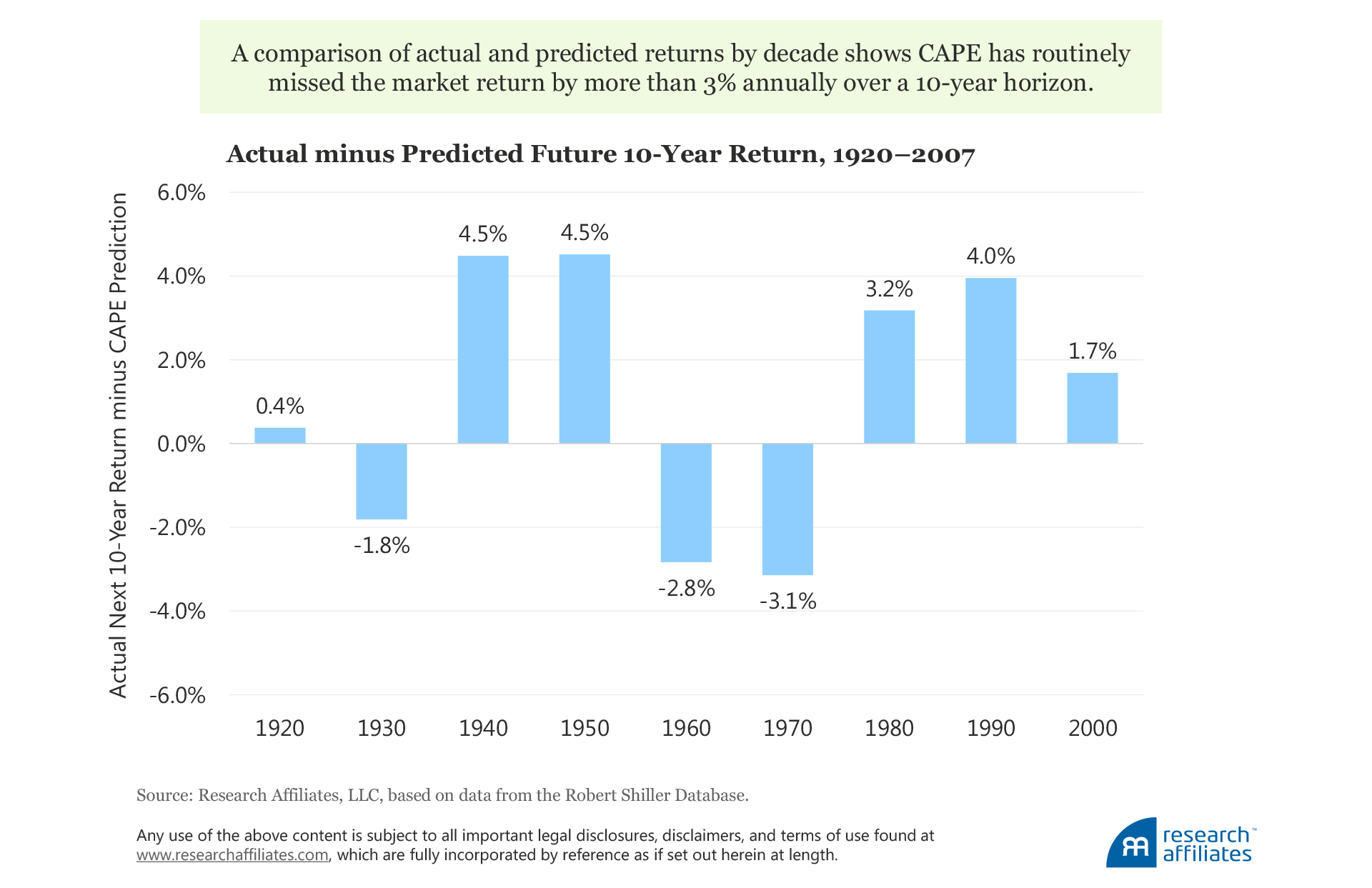
This relationship shows that future total returns are negatively, and significantly, related to the CAPE ratio today; or more simply stated, a high P/E multiple portends lower future returns. Let’s examine the predictions of CAPE in a rolling out-of-sample fashion, not by using the preceding equation, but by estimating the coefficients at the start of each period and comparing the predicted results over the next 10 years to the actual market return.
The difference between actual and predicted returns in each decade, beginning in 1920, shows that CAPE has routinely missed the market return by more than 3% annually over a 10-year horizon. For example, the 1970s value of −3.1% indicates that for predictions of return using CAPE made in the 1970s, the actual market return over the next 10 years was 3.1% lower than predicted by CAPE alone. Values closest to zero, such as 0.4% in the 1920s, indicate when the prediction was closest to what actually transpired in that decade.
Some may see the performance (or lack thereof) of CAPE as a tremendous failure, while others who appreciate the challenge in modeling expected returns will see it as a promising result. I say, it’s hard to criticize a model without another model to compare it to, so let’s next consider the performance of an old friend from 60 years ago, the Gordon Growth model, before reading too much into the CAPE results.
Old Friend: Yield and Growth
The Gordon Growth model (henceforth, the yield-plus-growth model to use terminology consistent with the AAI platform on our site) states that the return of an asset is equal to the cash-flow yield plus growth in future cash flows.
The most common implementation of the yield-plus-growth model is the starting dividend yield of the index and the long-term growth rate in real earnings per share. Yield, in yield plus growth, is defined as the dividend yield in each period, and growth as the long-term growth rate, which is trend earnings per share growth up to the start of the period. When we add the yield-plus-growth model to our decade-by-decade CAPE results, we find that CAPE initially had a great run, winning the five consecutive decades beginning in the 1920s, but lost three of the last four decades: 1970s, 1990s, and 2000s.
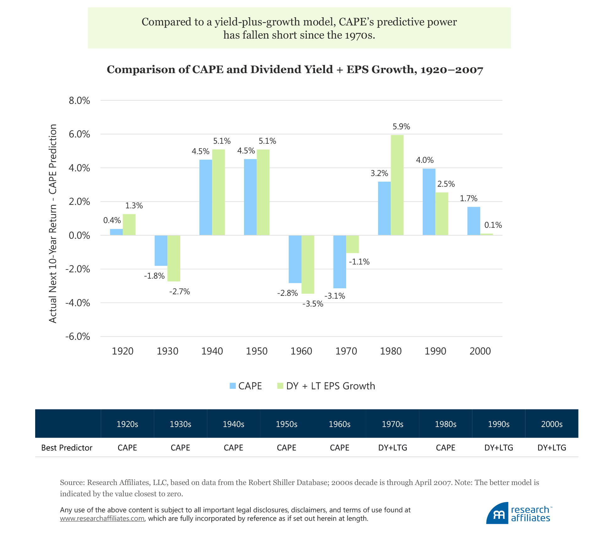
Investors who used the yield-plus-growth model over the last two decades would still have underestimated the actual real return of a market on a strong bull run, but would have outperformed the one-factor CAPE model. This finding is consistent with Cornell, Arnott, and Moroz (2009), who in studying the equity risk premium observed: “Because of the increasing importance of repurchases, the earnings growth model appears to be the preferred choice when using post-1980 data to estimate the unconditional risk premium.”
Research Affiliates Valuation- Dependent Model
Finally, let’s look at the Research Affiliates valuation-dependent expected returns model in which we include a mean-reversion characteristic as part of our long-term building-block forecast. For equities, CAPE is the metric we use to measure expectations in the expansion or contraction of equity multiples (our valuation-change building block). In the model we simply compare the current CAPE to a fair-value estimate:
Expected Return = Yield + Growth + Valuation Change2
The trick is to identify the fair-value CAPE, which is often assumed to be the long-term average of about 16. In recent research, Aked, Mazzoleni, and Shakernia (2017) find that the fair-value multiple for equities is time varying based on macroeconomic volatility, and that the reduction in macro-volatility over time has led to the fair-value CAPE going higher. The idea is that lower volatility makes investors more comfortable earning a lower risk premium, or taking on a higher CAPE.
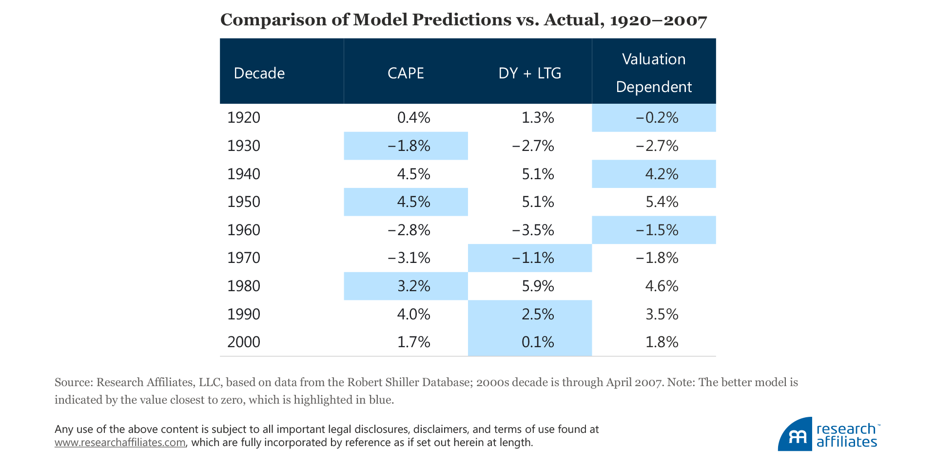
Although this is a great way to determine a fair-value discount rate, for simplicity, let’s use a straightforward fair-value estimate, which is a reversion halfway from current CAPE to its long-term average over a 10-year period. This method is a simplistic way of deriving a fair-value estimate from information contained in both the long-term average as well as from current market sentiment. A comparison of all three models shows that each has “won” in at least three decades from January 1920 through April 2007.
None of the three models is a “silver bullet” one-size-fits-all approach in all market environments. Each, if the one and only model used by an investor all the time, would induce model fatigue at one time or another.
Using Multiple Models
As an old saying goes, a man with a watch knows the time, but a man with two watches can never be sure. By having multiple models, have we simply muddied the waters?
If your goal in expectations modeling is to determine the exact return of an asset in the future, multiple models may, or may not be, useful. Trying to estimate an exact figure, however, is almost impossible to consistently achieve. None of the models discussed in this article would be a particularly effective approach for achieving this objective.
If your objective, as ours, is to use expectations as a mechanism for reducing the odds of a portfolio missing the level of return necessary to meet predefined spending needs, such as the 5% challenge in West and Masturzo (2016), multiple models can be extremely helpful. The use of multiple models allows investors to create portfolios based on different perspectives, similar to blending factor portfolios to gain particular exposures—the recent rage in equity investing.
Using each model, we can create a strategic asset allocation portfolio (called the “efficient portfolio” on the AAI platform) for varying levels of risk. Portfolios based on the yield-plus-growth model have an income focus, while those incorporating valuations adopt a mean-reversion perspective. Blending portfolio allocations based on different expectations models has the added benefit of reducing model risk inherent in any individual model, even these two models, which have some definitional overlap.
With those two extremes an investor is able to blend portfolios based on personal constraints (such as tracking error or investment beliefs about, for example, the richness or cheapness of assets) in order to construct a portfolio with the multiple perspectives that address their specific needs. This approach acknowledges that no single strategy is appropriate for all investors all the time by providing an extensible framework to meet the diverse needs of investors.
A Blend Is Better
With the newest release of our Asset Allocation Interactive platform, we introduce the functionality of viewing expected returns through a yield-plus-growth lens in addition to our traditional valuation-dependent model. Using each of the models, we show efficient allocations that maximize return for varying levels of risk. The two expected return models can be blended together, resulting in a blend of the portfolio allocations under each.
The performance of the one-factor CAPE model, which has underperformed other models over the past few decades, may or may not rebound in the future—we do not have a crystal ball. Nor do we know which of the other return expectations models will produce good results for investors. What we do know is that an assumption that any particular model is always the best one—and many investors take that approach with CAPE—will lead to model fatigue. We believe the most successful way for investors to meet future spending needs is to blend portfolios based on different models of return expectations.
Endnotes
1. A similar equation is in Siegel (2016). The coefficients change due to a different measurement time period.
2. If the building-block values are small, we can ignore the cross-product terms and simply add the building blocks.
References
Aked, Michael, Michele Mazzoleni, and Omid Shakernia. 2017. “The Quest for the Holy Grail: The Fair Value of the Equity Market.” Research Affiliates (March).
Campbell, Harvey, and Robert Shiller. 1988. “Stock Prices, Earnings, and Expected Dividends.” Journal of Finance, vol. 43, no. 3 (July):661–676.
Cornell, Bradford, Robert Arnott, and Max Moroz. 2009. “The Equity Premium Revisited.” Working paper (February).
Siegel, Jeremy. 2016. “The Shiller CAPE Ratio: A New Look.” Financial Analysts Journal, vol. 72, no. 3 (May/June):41–49.
West, John, and Jim Masturzo. 2016. “Take the 5% Challenge! (or The “Lloyd Christmas” Lesson).” Research Affiliates (October).
Copyright © Research Affiliates


