GMO: Investment Outlook (May 2016)

GMO: Investment Outlook (May 2016)

Keeping the Faith

by Ben Inker and Jeremy Grantham, GMO LLC

The past five years have been challenging for long-term value-based asset allocation. We do not believe this constitutes a paradigm shift, dooming such strategies in the future. The basic driver for long-term value working historically has been the excessive volatility of asset prices relative to their underlying fundamental cash flows, and recent history does not show any evidence of that changing. Outperforming the markets given that pattern requires either betting that the excessive swings will reverse over time or accurately predicting what those excessive swings will be. The former strategy amounts to long-term value-based investing, while the latter requires outpredicting others as to both what surprises will hit the markets and how the markets will react to them. Our strong preference is to focus on long-term value, despite the inevitable periods of tough performance that strategy will entail.

Introduction

It’s no secret that the last half decade has been a rough one for value-based asset allocation. With central bankers pushing interest rates down to unimagined lows, ongoing disappointment from the emerging markets that have looked cheaper than the rest of the world, and the continuing outperformance from the U.S. stock market and growth stocks generally, it’s enough to cause even committed long-term value investors to question their faith. Over the past several years, we at GMO have questioned a lot of things, including assumptions that we had held without much question for decades, but we have not wavered in our belief that taking the long-term view in investing is the right path and that in the long run no factor is as important to investment returns as valuations. In this letter, I’m going to talk about some of the reasons we continue to believe this so strongly.

Perhaps the first point to make on why we continue to stick to our beliefs is that this is far from the first period in which the patience of long-term value managers has been tested. A decade ago, we were all told that the great moderation had changed the rules of investing, making it safe to invest in risky assets without the margin of safety that used to be required. Less than a decade before that, we were all told that the internet had changed the rules even more profoundly, making anyone who was prepared to put money into boring REITs or TIPS in return for paltry mid to high single-digit real returns a fool for foregoing the hugely greater potential returns from investing in the loss- making companies that were someday soon to become massively profitable. As GMO’s portfolios
were positioned for the opposite in both cases, we got plenty of complaints from clients that we just didn’t get it. But the periodic struggles of long-term value investors far pre-date GMO’s founding. You can hear the frustration evident in John Maynard Keynes’s quote from the General Theory back in 1936: “It is the long-term investor, he who most promotes the public interest, who will in practice come in for most criticism.”1 I can’t tell you exactly what was going on in Keynes’s head when he wrote that, but to me it has all the hallmarks of someone who has just come back from a particularly trying investment committee meeting.

So this is certainly not the first period that has tested the faith of long-term value investors, but the fact that a style of investing has seen problems before is far from a guarantee that it will succeed in the end. While our faith is helped by the fact that this is not our first experience with misbehaving markets, the reason for our belief comes much more from a systematic study of history and the fundamental drivers of asset returns. The evidence is clear that asset prices are much more volatile than can be justified by the underlying fundamentals. This is the basic driver of the long-term returns to value- based asset allocation, and recent history, as painful as it has been for some of our bets, shows every bit as much excess volatility as the more distant past did. A world in which value-based mean reversion will not work in the long run is a low volatility world in which asset prices do not deviate from the slow-moving fundamentals that power financial markets. It is extremely hard for us to justify the last several years of market behavior through that lens, which leaves us confident that our strategy will work in the end.

Value has always been a risky strategy, particularly for those trying to run an investment business. The drivers of mean reversion are not hugely powerful at any given time, meaning asset prices and even the underlying fundamentals can move in unexpected ways for disappointingly long periods. It is a little glib to say that without this risk, it would be difficult for asset prices to get meaningfully out of line in the first place, but the reality is that the only way you can get really exciting opportunities for mean reversion is to have misvalued assets become even more misvalued before they revert to fair value. This is the catch-22 of value-driven investing. Your best opportunities will almost always come just at the time your clients are least interested in hearing from you, and might possibly come at the times when you are most likely to be doubting yourself.

Asset prices are too volatile

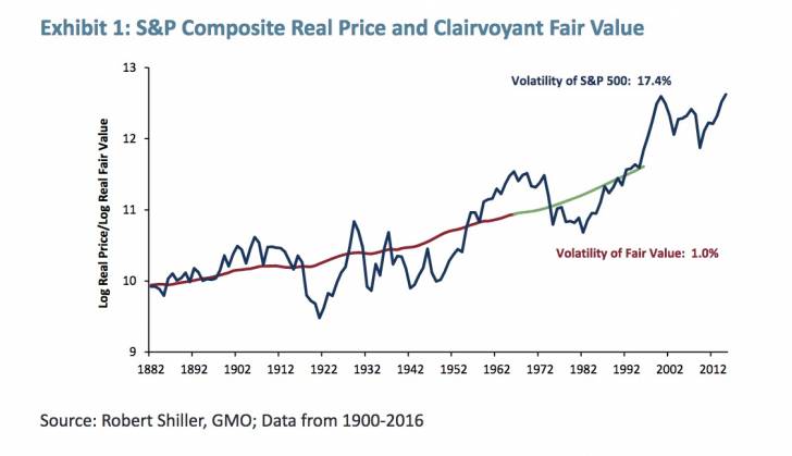
So, why do we believe that asset prices are more volatile than they should be? Robert Shiller, the Nobel Prize winning Yale economist who is the source of so much common sense wisdom on financial markets, did a simple but powerful test of this almost 30 years ago in a paper for Science magazine.2 Shiller noted that while we cannot know the future with any degree of certainty, we have no such limitation when it comes to the past. He looked at U.S. stock market prices and dividends back to the 19th century and came up with a “clairvoyant” fair value estimate for the market based on the actual dividends that were paid over the next 50 years. This analysis, which is reproduced and updated in Exhibit 1, made the following important point.

The volatility of U.S. stocks since 1881 has been a little over 17% per year. The volatility of the underlying fair value of the market has been a little over 1% per year. Well over 90% of the volatility of the stock market cannot be explained as a rational response to the changing value of the stream of dividends it embodies. This means that the volatility is due to some combination of changing discount rates applied to those cash flows, and changes to expectations of future dividends that turned out to
be incorrect. It is difficult to determine exactly which has been the driver at any given time, but there doesn’t seem to be a lot of evidence for changing discount rates having been a major force. Even in the most extreme overvaluation in U.S. stock market history, the 1999-2000 internet bubble, none of the investors we heard explaining why the stock market was rational to have risen to such giddy heights explained it on the basis that future returns should be lower than history.3

It’s somewhat harder to dismiss the changing discount rate argument as a partial explanation for today’s high equity valuations. Unlike 1999, bond yields today are strikingly low, and so if stocks should be priced by demanding a risk premium off of a risk-free rate (an idea that my colleague James Montier, for one, rejects4), we could understand why stock valuations might be high today relative to history.

But if a changing discount rate had historically been a significant driver of stock market volatility, we would expect to see some explanatory power for bond rates in explaining changes in stock prices. This connection, at least historically, is almost completely absent, as Exhibit 2 shows.

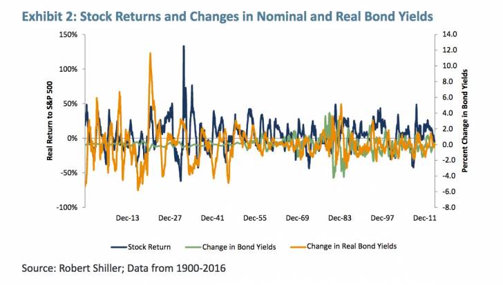
If this chart looks like a complete mess, that’s because it is. The R2 of changes in nominal bond yields to explain stock market returns is 0.02, and for changes in real bond yields it is 0.01, although because the beta on the factor has the wrong sign (higher real bond yields imply positive stock market returns), it’s hard to even give credit for that 1% explanatory power. In either case, we cannot explain any meaningful part of the excess volatility of the stock market historically as coming from the piece of the discount rate that can be observed.5

Predicting surprises is hard

The fact that markets are more volatile than they need to be certainly doesn’t mean you can’t try to predict and profit from those “unnecessary” moves. But how do you predict them? To a very significant degree, markets in the short term are driven by “news” – events that would have to be predicted ahead of time to properly guess what the markets will do in the future. This task is complicated by the fact that even given an accurate prediction of news or surprises, which for this purpose are synonymous, predicting the actual response of the market is surprisingly tricky, because the connections between data and events and stock market performance are often unintuitive.

One point to recognize is that predicting news may be possible, but it certainly cannot be done by the median participant, because if the median participant predicted it, it wasn’t news in the first place. But the market consensus is generally dreadfully unimaginative in any event. To take a relevant example, probably the most important single piece of macro information that investors would like to know ahead of time is the timing of recessions. Exhibit 3 shows the historical ability of economists to predict recessions in the form of predictions of the following year’s GDP growth.

Economists have entirely failed to predict any of the recessions we have had in the time since consensus forecasts were available, and this may actually be an unfairly easy test. In principle, economists could have successfully predicted recessions and had the information be useless for investors because the market had already priced in the probability. But every single recession – and indeed pretty much every surge and dip in GDP growth over the past 40 years – has been poorly predicted by Wall Street economists.

Figuring out what to do with surprise

But let’s assume that you could actually predict surprise, and in a piece of data widely known to move markets. For this purpose, I’m going to use U.S. payroll data. We get new payroll data every month and we have a record of the consensus forecast going into each release since 1997. So we can see the impact of properly predicting the surprise in payroll data going back almost 20 years. Over a day, the impact is clear. A positive payroll surprise leads to an average return of 0.24% for the day, while a negative surprise gives an average return of only 0.02%. This seems perfectly reasonable, but what is peculiar is what happens over a longer period. We might readily expect that the bulk of the excess return to the data would come out in the day it is announced, but the real world is actually not even that kind. Exhibit 4 shows the one-day, one-month, six-month, one-year, and three-year returns. You can see that for a day, the impact of a surprise on payrolls is material. As the time horizon lengthens, the “importance” of the surprise disappears quickly and then, oddly, actually shifts sign! This is a pretty striking result. The market does indeed rise when we get a positive surprise on payrolls, but as time passes, the news turns out not to actually matter for the true fair value of the stock market, or at least not in the manner traders might have originally assumed.

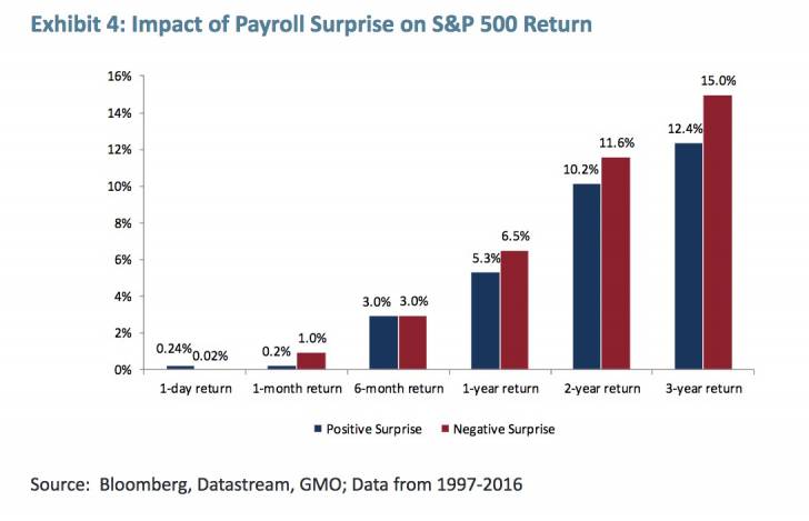
It’s a little hard to explain the one-month and six-month data consistently – why would the impact of surprise be negative over the first month and then positive over the next five? But the pattern over one to three years certainly suggests that, all else equal, you’d rather own the stock market in the few years after a disappointment in employment than after a positive surprise. Does this mean that investors should sell when the payroll data surprises to the upside? Probably not. It’s not a particularly huge effect and there are many possible reasons why it could have wound up looking odd. But it does mean that if you are planning to make money by predicting payroll data better than the other guy, you’d better be quick about it, because there is no actual evidence that strong payroll data actually increases the value of the stock market in any lasting way.

The lasting power of value

By way of contrast, Exhibit 5 shows the impact of the market being cheaper than average or more expensive than average on the day of the payroll announcement over the same time period.

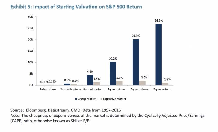
This chart again starts on the day payrolls are going to be announced. For that single day, the performance of the market seems to actually be negatively correlated with cheapness. On that first Friday of the month, being expensive means that the market rises 23 basis points, whereas if it is cheap, it is flat.6 But as the time horizon lengthens, the importance of valuation rises more and more. There are actually a couple of problems with Exhibit 5, which I don’t love, but for the sake of complete comparability with Exhibit 4 I used it anyway. One problem is that it’s actually a reasonably small sample of data – a total of 232 events in which we had payroll announcements since 1997. The other is that all of the dates were Fridays, in fact the first Friday of the month (with a couple of exceptions for holidays). As it turns out, “Payroll Friday” has been a pretty good day for the S&P 500, with an average return of 12 basis points, or 35% annualized. Given that the actual return for the S&P 500 since December 31, 1996 was 7.4% annualized, which is an average of three basis points per day, it turns out payroll Fridays weren’t ordinary days. To see the basic power of value, it would be better to use all days, and over a longer period.

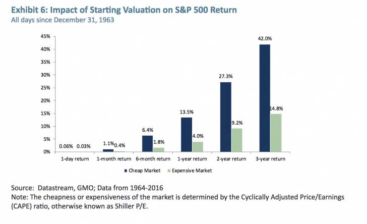
Exhibit 6 shows the value effect for all days going back as far as we have daily prices for the S&P 500, which is the end of 1963.

It’s a striking exhibit. Over one day, being cheap earns you an average 6-basis-point return versus 3 basis points for an expensive market. But, as the time horizon lengthens, the advantage for cheap markets grows. Actually, it’s even a little cooler than that.7 If we look at the daily impact of having started cheap versus expensive over the various time horizons, we get the following in Exhibit 7.

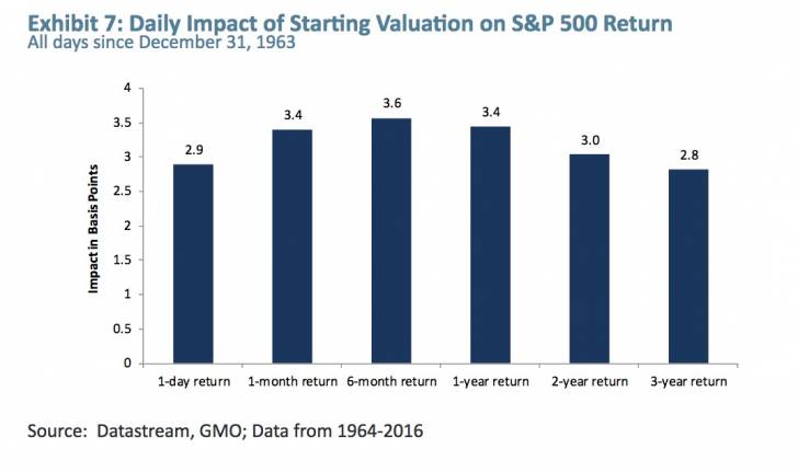
Over a given day, the impact of being cheap versus expensive is small – just under 3 basis points. But it persists. The importance of having been cheap on the first day of the period is also around 3 basis points per day for the next month, and this is more or less the same as it is over the next six months, one year, two years, and three years.8 Value has been referred to as the gravitational pull of the financial markets, and with good reason. Gravity is far and away the weakest of the four fundamental forces of nature, but it is unique in that it always acts in the same direction and does so over arbitrarily

And this is the basic virtue of taking a long time horizon. If you want to make money over a day, by all means try to predict the payrolls number. If you do it better than everyone else, you can make far more in that day than you ever could with value. But predicting surprises is hard. Most people who attempt it will fail. And the funny thing history teaches us is that most things that seem important at a given time – who wins an election, what this quarter’s or year’s earnings turn out to be, whether there is a recession or not – dissipate in importance over time if they ever truly mattered in the first place.

“Important” data often doesn’t matter

One of the most striking demonstrations of the tendency of seemingly important data not to matter is the relationship – or lack thereof – between equity returns and GDP growth, which we have mentioned before. Exhibit 8 shows the relationship between GDP growth and stock market returns for the developed markets from 1980-2015.

Investors all over the world “know” that GDP growth is an important determinant of stock market returns. Generally speaking, the complaint by investors is the difficulty of predicting GDP growth in time to invest accordingly. But the analysis below sidesteps that problem as it assumes complete clairvoyance. It answers the question as to how you could use the information of perfect foreknowledge of GDP growth across the developed world over the last 35 years to make money in the stock market.

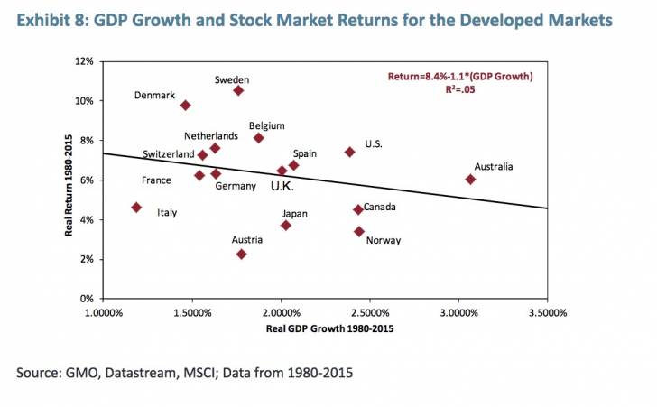
And the answer is that you could indeed have used the knowledge to make money, although not in the expected way. The lowest growth quartile of countries outperformed the highest growth by 2% per year, enough to make a dollar invested worth 85% more in the slow growers than the fast growers. This pattern is not unique to this particular time period. On the longest run of history we have for a wide group of countries, the Dimson, Marsh, Staunton dataset from 1900, we see the same pattern (although the data they kept is GDP per capita instead of total GDP). This is shown in Exhibit 9.

9 Okay, I have to admit this isn’t strictly true. Because gravity propagates at the speed of light, the distance over which gravity can influence objects is limited by their distance and the age of the universe, so two objects on opposite sides of the visible universe are too far apart to have any gravitational impact on each other. This is almost certainly a case of taking an analogy too far, so I’ll stop now.

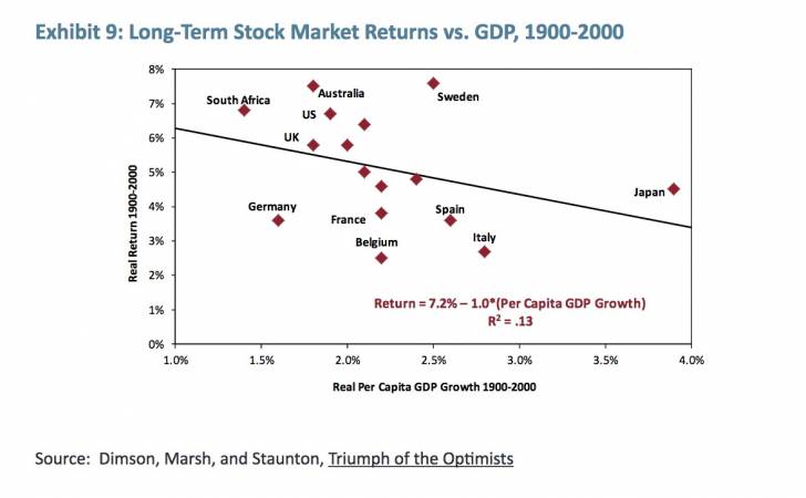
Again, over the last century or so, knowing which countries would have grown fastest was not actually useless for predicting returns, but properly utilizing your extraordinary foreknowledge required the unintuitive step of systematically buying the countries that would grow the slowest. Was there any information that would have been useful to know over the period? Yes. For the clairvoyant investor, it definitely seems to be the case that knowing which countries would be invaded or suffer a civil war was a plus in the long run, but, at least since 1980, there was a piece of information knowable to even the non-clairvoyant among us that would have been extremely helpful in predicting future returns. Exhibit 10 shows the relationship between starting valuation – in the form of a cyclically-adjusted earnings figure – and returns over the next 35 years.

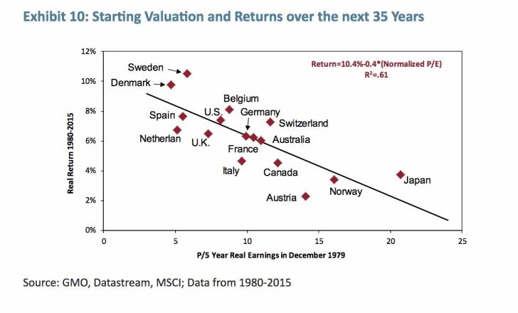
The correlation was a stunning -78%, and the benefit to that knowledge was profound. The cheapest quarter of countries outperformed the most expensive quarter by an enormous 5.1% per year for 35 years. A dollar split among those countries would have turned to 26.4 dollars in real terms, while a dollar invested in the expensive countries would have grown to only 4.9 dollars. And that is from information that was actually readily knowable at the time, no clairvoyance needed.

Time horizon for bond investors

The short-term importance of “surprise” in the bond markets is every bit as important as in stock markets, if not more so. But the unyielding10 mathematics of bond returns also means that as the time horizon lengthens, the importance of starting yields rises inexorably. Exhibit 11 shows the impact of payroll surprise on the Barclays Capital 7-10 Year U.S. Treasury Bond index.

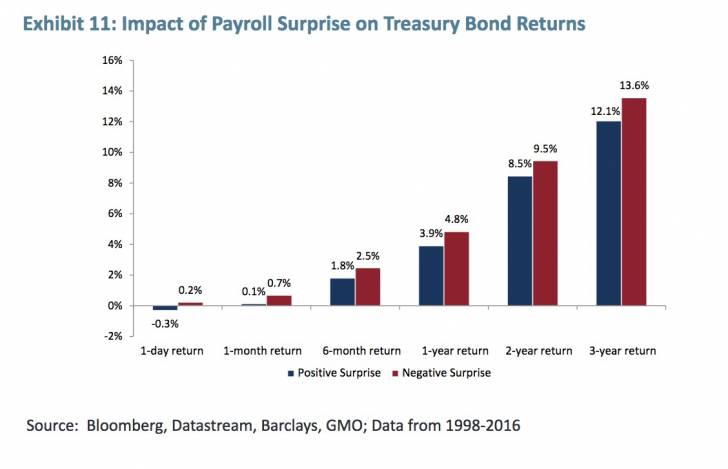
Successfully predicting payroll surprise has meant a 0.5% swing in the one-day return of Treasury notes, which is pretty extraordinary given the low volatility of the bond market. And, unlike in equities, the importance of the surprise hasn’t switched signs over time. On the other hand, bonds are called “fixed income” for a reason. As the time horizon lengthens, the importance of the starting yield of the bond becomes overwhelming, as it must, as we can see in Exhibit 12.

It is universally understood (I hope) that a 10-year Treasury note yielding 1.84% held for 10 years will give a return pretty close to 1.84%.11 It is not quite so widely known that the rate of return of a dynamic portfolio of such bonds – a “constant maturity strategy” – is also pretty well fixed for certain time horizons. To take the Barclays U.S. Aggregate Bond index (Agg) as an example of a dynamic portfolio, with a duration of a little over five years and a current yield of 2.17%, the range of possible returns over the next seven years is not very wide. We are not guaranteed to get 2.17%, but the return if the yield were to gradually drop to zero over that period would be about 2.9% per year, and if the yield were to gradually double, it would be about 1.5% per year. No matter what happens to yields over the next seven years, returns are going to be something pretty close to 2.17% on the Agg. There is simply no way for it to give a return close to the 7.7% the index has returned on average since its inception in 1975. A significant part of the reason why valuation has mattered so much for equities over the years is because valuations have been mean reverting. Yield is far and away the crucial factor for returns on high quality bonds, whether or not yields mean revert.

In the short run, any bond, including the negative yielding ones common in Europe and Japan at the moment, can give a significantly positive return due to news that causes yields to fall further. In the longer run, a 10-year Japanese government bond yielding -0.09% is going to wind up giving a return of around -0.09%, no matter what surprises the Bank of Japan unveils to the markets. While there are investment problems that a return of -0.09% can help solve, there aren’t many of them. Given how many government bonds are trading at similar yields, this puts much global government debt in the odd position of being potentially an interesting short-term speculation, but close to useless for long- term investors.13

Conclusion

So, why should anyone keep the faith as a long-term value investor? It is not enough to say that the alternatives are worse, because one possible alternative is to go passive and stop playing the game. We hold fast to our faith because, while the performance of value has been lousy over the last few years, there is little or no evidence that this is due to the markets somehow becoming more efficient. The performance of risk assets in the first quarter of the year, with global stocks falling 11% in the first six weeks only to turn around to rise 13% in the next six, has all of the hallmarks of a market obsessed with short-term surprises, not efficiently discounting the pretty stable stream of cash flows that most asset classes actually give. Efficient markets would show little volatility because the underlying fundamentals are stable. Today’s markets, whatever else they may be, are clearly not efficient in that sense. Hyperactive central bankers and jumpy investors unable to decide between reaching for yield or running for safety may be a significant annoyance for long-term value investors, but we should not forget that their actions also create the very opportunities that such investors need to outperform in the long run.

1 John Maynard Keynes, General Theory of Employment, Interest and Money, 1936.

2 Robert Shiller, “The Volatility of Stock Market Prices,” Science (January 2, 1987).

3 At the time, the Glassman and Hassett “Dow 36,000” piece did make the argument that equity returns should be lower than history, but did so within their argument that the market deserved to trade three times higher than the level at which it was actually trading.

4 See, “The Idolatry of Interest Rates, Part 2: Financial Heresy and Potential Utility in an ERP Framework,” August 11, 2015. This white paper by James Montier is available at www.gmo.com.

5 The other piece of the discount rate for stocks is the equity risk premium part. As this can only be measured by looking at the valuation of stocks and backing out an implied risk premium over bonds (or alternatively ignoring bond yields and just looking at the valuations of stocks), “explaining” the volatility of the market in this fashion amounts to saying “changing stock valuations explain 100% of the change in stock prices that is not justified by changing fundamentals.” Tautologically true, but completely consistent with saying that stock prices are hugely more volatile than the underlying fundamentals justify.

6 This isn’t actually inconsistent with the returns on the payroll surprise chart even though the average return looks a few basis points lower than on Exhibit 4. As it turns out, since 1997, there have been a few more negative payroll surprises than positive surprises.

7 Cooler for value nerds at least. Possibly, the following exhibit will give you less of an “oooh” shiver than it did me.

8 This exhibit shows the “cheating” impact of valuation, in that the definition of cheap versus expensive is defined over the entire time period, not history to date. If you did the “no cheat” version, the daily impact does shrink a bit over time, from a maximum of 3.7 basis points on day one, to 2.5 basis points over the next year, to 2 basis points over two years, and 1.7 basis points over three years.
large distances.

9 For markets, the impact of value is small over a single day – since 1964, being cheap led to a positive 0.015 standard deviation event above average in that day – but as the number of days grows, the impact becomes more and more material.

10 Sorry, couldn’t resist.

11 The primary uncertainty comes in the rate of return that will be earned on the coupons earned along the way.

12 To achieve a return of 7.7% for the index over the next seven years, yields would have to fall to approximately negative 17% at the end of the period, ignoring roll and convexity effects. While recent history has shown that negative interest rates are indeed possible, -17% really does seem to be well lower than can be imagined.

13 The bonds are guaranteed to give little or no return in nominal terms. In the event that inflation runs significantly below zero over the next decade, the return above inflation could well be positive, but it is worth noting that neither inflation swaps nor economists’ forecasts imply that investors actually believe that inflation will turn out to be negative.

Disclaimer: The views expressed are the views of Ben Inker through the period ending May 2016, and are subject to change at any time based on market and other conditions. This is not an offer or solicitation for the purchase or sale of any security and should not be construed as such. References to specific securities and issuers are for illustrative purposes only and are not intended to be, and should not be interpreted as, recommendations to purchase or sell such securities.

Copyright © 2016 by GMO LLC. All rights reserved.

Read/Download the complete report below (the Jeremy Grantham portion follows Ben Inker's commentary):

Gmo Quarterly Letter by dpbasic