


Wayfaring on CAPE’s Edge
by Salil Mehta, Statisical Ideas
As U.S. equity levels define new record highs, we are treated to market observers who again debate the significance of the high cyclically-adjusted P/E ratio (Campbell and Shiller’s CAPE). This debate generally revolves around the predictability of 10-year future returns, based upon the decile level of CAPE. And a seemingly straightforward math exercise is then further complicated by pundits, who seek to explain nuances of the predicted results, particularly since the current top-decile CAPE generally reflects fairly weak long-term equity returns. A probabilist looking at this CAPE situation would instead want to focus inward. Wanting to better understand the statistical robustness of this modeling ratio, as well as any gaps in how people interpret its results.
Probability theory has some caution to lend, even in what appears to be a simple case of studying the differences in decile factor returns. Evidently it seems that nearly one and a quarter century worth of annual CAPE data is a very considerable sample with which to work. Most would conclude that this number would equate to a per-decile sample size of just more than a dozen. But as we’ll later see, this is not quite accurate. There are still some probabilistic nuances that one needs to accept and analytically reconcile, prior to going further downstream as economists and pundits have, in explaining the at-face-value results.
In this web log article, we will seek to understand the rarity and timing of our high CAPE. And we will discuss what this means, as one attempts to interpret CAPE. First we should realize that U.S. earnings are calculated most carefully on an annual basis, not in a higher frequency such as quarterly or monthly. Pricing data is of course something that can be measured more frequently than daily. But given that both price and earnings are almost equally volatile, the sampling of data should is best aligned on an annual basis, in order to match the source of CAPE variance from both the numerator and denominator. In a new NBER working paper, Mr. Bunn and Professor Shiller explore optimization of another time horizon (i.e. those of future returns). The relationship should be convex, and (I asked them about this) they disagreed about this focus and highlight a straight -to sometimes choppy- negative relationship between the time horizon and statistical significance (as measured by p-value). Please refer to those working paper charts to have a closer look.
Next we have to remove some sampling degrees of freedom (dof) to account for the rationale of sampling. This is a core theme throughout the Statistics Topics book (top of this AR list, and Professor Shiller also acquired a copy), that mathematical models are only as good as the logic behind the formula assumptions. We aren’t simply asking for the probability of seeing a portion of the distribution (e.g., a high CAPE, from within a probability distribution of CAPE values), but rather given a history of CAPE values, how likely would we now see a high CAPE? So we can not include the probability of the entire history, if we also seek the probability given that same history. This idea mixes with the preferred underlying modeling assumption that we might have identical and independent (iid) drawings of CAPE, from one year to the next. Now iid isn’t necessarily violated even though we have a constant overlap of 9-years of every 10-year window, for each year that we roll forward through time. But iid is violated at the boundaries of the partition (and later we’ll see violations through serial correlation as well); we will need to see some probability modifications to partition the time series multiple times. Lastly there is clear censoring of the initial decade of real price data, as only earnings were being collected then, for the initial denominator’s cyclical calculation.
To begin with, the initial CAPE data could have started with nearly 175 years of data, but Professor Shiller and his colleagues had censored a number of initial decades of the Railroad transport era stating they were too volatile. So now we are left with a starting CAPE data set of 143 years, but then with the probability adjustments noted, we are now left with is a sample size brought half-way down to 100. Now there is some serial correlation (we have a Spearman-r calculation on the decile values of nearly 0.8) in the CAPE data. So we can not simply take the standard deviation of the annual CAPE values, and determine how relatively far away the current CAPE is from the historic average.
For example, a 6-sided dice (with an average face-value of 3.5) always has a 1/6 chance of landing on 6, regardless of whether the previous roll was a 5, or a 1. On the other hand, a CAPE of 25 in a given year is more likely to happen if the prior year’s CAPE was 20, versus if the prior year’s CAPE was 5.
So the probability model needs to be crafted in two parts, in order to provide the best estimate. The first part is the probability of having a CAPE that breaches its typical “upper-bound” of 22 to begin with. This upper-bound excludes exactly 1/7 of the data (the extreme CAPE values seen near 1929, the majority of the past 18 years, plus 1965, 1966, 1899, 1902). Then we calculate the new conditional probability that once the value of 22 is touched, what is the probability of then seeing a CAPE value of 25 as the CAPE stochastically vibrates about after hitting the 22 upper-bound? Later below we will refer to this second part as a "detached statistical unit". Note the 25 value is for a current extreme CAPE estimate since the actual 2013 CAPE was 21. These two probabilities together provide an answer that we have about a three percent probability of seeing the current high CAPE. Certainly once every multiple decades.
The inexperienced manner to have calculated this probability is to simply take the 17 CAPE average (with a 6 standard deviation) over its full 133-year history. Using a normal distribution, we would then incorrectly state that a 25 CAPE would have a near 10% probability of occurring (much higher versus our refined technique). Our sophisticated approach also comports to the true extreme CAPE value that we have, which would reside the outer-edge of the top-decile (10th decile). This also suggests that we should be even more careful when interpreting the results, of predicting the 10-year future returns, based upon the current CAPE state.
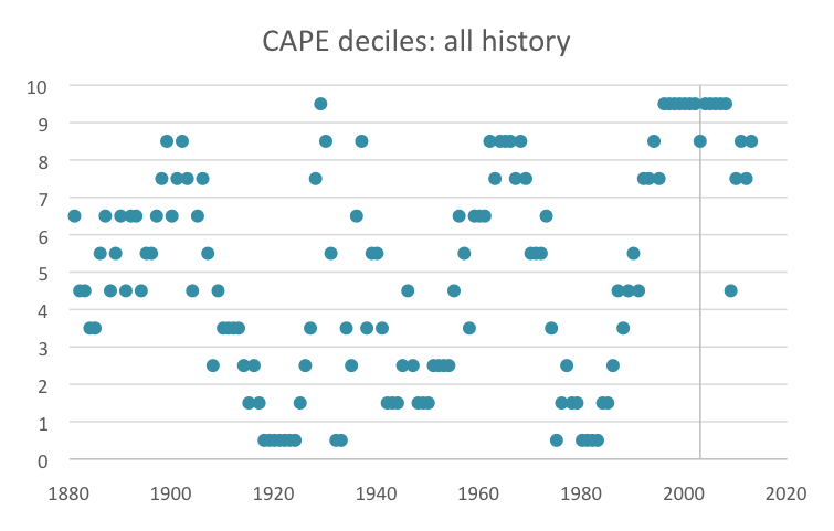
Now let’s look now at the entire CAPE historical time series, but here plotting the decile values. The 2003 line marks the time beyond when the 10-year future returns are not fully available. So even if the CAPE were in the top decile subsequent to 2003, we could only use the years prior to and not after 2003, in order to gauge the available set of historical 10-year future returns.
We notice the serial correlation in this non-parametric (using ranked data would eliminate a robust model) chart above. For example, CAPEs generally don’t jump directly (in one year) in either direction, between the 1st decile, and 10th decile. We also notice that roughly 40%, of the top-decile years, occurred in just the past decade. So despite having started with nearly 175 years of data, we have been reduced to a 10th decile size of only about 7 (from which to differentiate this decile’s 10-year future returns). This significantly weakens any statistical conclusion coming from this sort of decile analysis, and even Professor Shiller's work recognizes that in his justifcation of natural-logrithmic return conversions particularly in the early years of the data set. He and Mr. Bunn attempt to rank the data based on other fractions as well, arbitraily at times choosing tertiles. I also asked them about this and was agreeingly told "the choice of tertiles is admittedly arbitrary", and indeed the focus of how it was still chosen was to keep the relationship sample size manageable.
Now we’ve been in a near continuous 10th decile CAPE environment, for more than just the past decade, but closer to 18 years. We can see this in the chart above, and note this streak starts just after 1994 when CAPE touched 22, for the first time in about 3 decades. So we have to consider in our modeling rationale that the past two decades must be just one detached statistical unit. And with it, we’ve then wiped out the complete 10th decile sample, save for just one remaining year: 1929!
How good would this decile-style factor analysis have contemporaneously worked through history, anyway? We focus on when economists most-mention as the previous high-CAPE signals: 1929, 2000, and 2007. It turns out that these previous examples were not highly fool-proof. In 2 of these 3 periods, one would have been badly burned by underweighting U.S. stocks, using this 10th decile CAPE signal. The 3rd period, one would have been more lucky than smart to have used it.
Let’s now jump into the time machine, and go back to 1929. Here is the CAPE decile time series, seen in 1929.
True, U.S. equities did fall after this signal. It’s also true is that the 10th decile sample size, pre-1919 was just 4. So one would have been a good deal lucky than smart to have staked his or her asset allocation strategy, at the time, on just the CAPE signal. Also note that those 4 other years were at the turn of the 20th century. Yet in the top chart above, those CAPE values today are not 10th decile, but instead 9th decile and even 8th decile.
Now let’s fast forward in time, to 1994. Here one sees a little more timing diversification of 10th decile CAPEs, across the history until then. We also see a sample size pre-1984 that is roughly 10. So clearly this should be a much stronger signal to underweight stocks, versus the lucky signal experienced in 1929.
We know how this story unfolds. Despite the U.S. markets having a 10th decile CAPE in 1994, equities and CAPE both continued to audaciously rally. For another 6 years! For those who today chose to cherry-pick the year 2000 as the CAPE signal for their trading strategy, they are providing a false backtesting sense of how the contemporaneous signals developed. Since their trigger was actually badly mistimed by coming on 6 years earlier, in 1994.
So of course these extreme CAPEs should be suggesting very weak 10-year future returns, not necessarily short term turns in the market (but again we need to understand the associated statistical confidence). Forward to 2004. The chart below looks similar to today’s all-inclusive time series (see topmost chart). As we noted in the prior illustrations, in 2004, much of the 10th decile CAPEs were since 1994. So those 10-year future returns, that the CAPE in 1994 suggested would be very weak? Actually they were a nice 150%; so they were not weak at all.
With the same 10th decile signal occurring here in 2004, what if one does underweights U.S. equities again based on this CAPE signal? The 10-year future returns since 2004 were ok, cumulatively about 80%. That doesn’t sound like a disaster. The real disaster would be that this CAPE decile signal, to underweight the markets, came three years early. And one would have miserably sat through an underweighted portfolio as the market took off, through 2007. This exercise of having false signals isn’t just a matter of using 10th deciles, or arbitrary CAPE values (e.g., 25).
To be clear, having extremely high CAPE values proves little, with statistical confidence. Some economists tend to agree with that for this data set. Poor modeling can be costly (note these various market-timing articles here, here, and here). And such naïve speculation sows the seeds of manias and bubbles. In 1997, the CAPE made a record high of 28, finally eclipsing the 1929 CAPE of 27. The CAPE has not only risen for the three prior years, since 1994’s upper-bound CAPE, but in 1997 it was at an extreme value. Was it “irrational exuberance”? Not at all, through the eyes of a probabilist. And the market, as we all know, continued to rally another three years! Being underweight U.S. equities, based on the 10th decile CAPE signal, would not have been smart - but rather agonizing. That story ends with the market continuing to define new highs, in the later part of the 10-year window ending in 2004.
Here we are at the familiar dance, once more. Now the year is 2014. The CAPE is not only near the 10th decile, but it is just shy of the most extreme levels at which it has ever been. As we know, CAPE has only previously reached at least these “lofty levels”, in 1929, and about half of the prior 2 decades. We are simply wayfaring on the edge of CAPE. It is important to repeat that there is no statistical confidence that this 10th decile CAPE value, implies a meaningful signal that we are due for an extraordinarily weak, 10-year future returns. We would have made a mistake to stake our claim on this signal, during parts of the mid-1990s, and again in 2004.
So we show in this article here that there is statistical difficulty in interpreting the meaning of extreme CAPE values. The unchartered area of these values makes probability analysis an imperative prerequisite for this debate, yet next to impossible for most analysts to perform. There are dof adjustments that are needed to account for the upward stochastic channel, which we noted occurred initiating in 1994.
Leading financial economists are now preferring the idea of introducing exogenous factors, to nicely explain the recent high CAPE values. Though probability modeling makes that a lower priority thing to do at this stage. Instead we revert to our understanding (shown in a Businessweek Chart of the Day) of the increasingly volatile earnings picture, in recent decades, as our primary mathematical consideration. And whether in such case or anyway with exogenous factors, the statistical usage of these explanatory variables would severely diminish the sample size of 10th decile results for backtesting purposes.
On a final note, we discuss the probability idea that we might be on an elevated CAPE plateau, as we peer across the historical charts shown above. To start, this would be unusually difficult to model in this case, even using the actuarial credibility analysis designed to address such a question. We do know that we are at least temporarily at this high CAPE (regardless of how) and that the modeling of 10-year future returns -predicted by CAPE- is still not clear-cut.
To understand the recently ever higher CAPEs, first let’s look at the other end of the decile spectrum. Today when we look back across the entire CAPE history, we see 1st decile values in the years near 1920. Also if we went back in time to 1929, the contemporaneous 1st decile values were also in most of those same years near 1920. The same can be said for the 1st decile values near 1980. But as we see in the turn of the 20th century, and again in the mid-1960s, the current 8th decile values were (at that time in the past) 10th decile values. This suggests that were are creating new record high CAPE values, which mostly crowd out the historic 10th decile values. And we can see in the topmost chart, that the lowest decile in the past two decades is not the first decile, but rather only the fifth decile.
Posted 1 week ago by Salil Mehta