Models Should Be Simple, But Not Too Simple

The Evolution of Optimal Lookback Horizon

With four parameters I can fit an elephant and with five I can make him wiggle his trunk.
~ John von Neumann

We’ve previously written about the potential for even “simple” investment systems to be deceptively complex.  Here is one example.

Many asset class rotational systems are optimized on lookback horizon (to our observation, most use 120 days), so we thought it would be interesting to investigate the evolution of optimal lookback horizon through time. This allows us to put ourselves in the position of an analyst at different points in history and try to speculate on the choices he might have made given the information at his disposal then. It’s important to conduct this sort of exercise because if, in looking back at past optima, an analyst might have chosen to use wildly different lookbacks at different points in history, it might call into question the stability of your choice of lookback today.

To perform this analysis we individually tested momentum systems with lookback horizons from 20 days (~1 month) to 260 days (~1 year) in increments of 20 days on a 10 asset class universe (ETF symbols DBC, EEM, EWJ, GLD, ICF, IEF, RWX, TLT, VGK, VTI back-extended with index data).  In order to isolate lookback horizon and minimize the potential impact of varying the number of holdings, we averaged the results across independent simulations for systems holding top 2, 3, 4, and 5 assets.  For example, we ran systems with top 2, 3, 4, and 5 assets using a 20 day lookback, and then averaged the results for a composite performance at the 20 day horizon.

Astute readers will note that this is almost the equivalent of a rank-weighted portfolio of five assets – almost because in this case the top 2 assets receive the same weight. In a rank weighting scheme, each asset carries a weight of:

The term in the numerator with rank raised to -1 signifies that the ranks are sorted such that higher ranking assets have a higher absolute rank, so the top asset out of 5 assets has a rank of 5, not 1. The weighting scheme is a way of expressing the view that assets with higher momentum have a relatively higher expected return over the next period, but where the magnitude of the momentum differential carries no information. In our experiment the ranks work out to:

Top 1 and 2: 28.6% each
3rd ranked: 21.4%
4th ranked: 14.3%
5th ranked: 7.1%

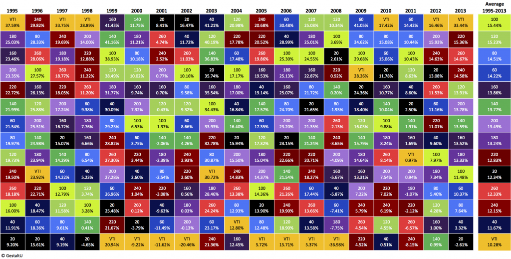
Figure 1. shows the calendar year performance of systems constructed with each lookback horizon, as well as the U.S. Total Stock Market index (Vanguard ETF symbol VTI).

Figure 1. Calendar year returns for momentum systems using different lookback horizons
Source: Bloomberg

First note the column on the right, which shows the cumulative return to each of the lookback systems over the entire period. The 100 day lookback delivered the strongest performance, while the 40 day system lagged. Interestingly, all of the systems exceeded the performance of U.S. stocks over the full 19 year period, though the S&P turned in top performance in 6 years, or over 30% of the time. Of course, it also turned in the worst performance in 8 years, or 42% of the time.  And there’s the rub. You see, while US stocks turned in positive performance in more than 80% of calendar years vs. 70% positive years for the momentum systems, the worst calendar year performance by any momentum system was -11.5% for the 60 day system in 2001, while the worst calendar year for US stocks was 2008, when they lost 37%.

Momentum systems in general delivered a narrower distribution of outcomes, especially on the downside.  We’d call these results pretty compelling at first glance.

Of equal interest, notice the dispersion in performance across the momentum systems from year to year. While the 100 day system was the peak performer on average over the entire history, it ranked near the bottom for the first few years, and its performance was also below average for the most recent two years. That said, keen observers will notice a potentially interesting performance ‘plateau’ that crests near the 100-120 day mark, and slowly decays as the lookback horizon moves further away in both directions.

Figure 2. illustrates how the top lookback horizons evolved through time by showing the cumulative annualized performance for each system through the end of each calendar year. Interestingly, an analyst investigating a simple momentum based asset rotation system in the late 1990s might have been forgiven for concluding that the concept was a bust, as U.S. stocks crushed every momentum system we tested from 1995 to 2000 on a cumulative annualized basis.

Figure 2. Cumulative annualized calendar year returns for momentum systems using different lookback horizons
Source: Bloomberg

It’s also interesting to note that the top performing lookback horizon over the entire testing period, 100 days, didn’t even creep into the top half of cumulative performance until 2002 – after the bear market. Also, the 60- and 80-day systems looked pretty grim until 2008, ranking near the bottom most years. However, in 2009 they did a better job of identifying the change in trend off the bear market low and, as a result, they leaped from the bottom quartile to the top quartile in short order, and remain there to this day.  Simply stated, if our lookback horizon is too long, we are likely to be adversely effected by rapidly deteriorating bear markets similar to 2008-9 (notice the drop in the 240-260 day lookbacks in figure 2.).  On the other hand, if it’s too short, we are likely to miss out on bullish reversals (which can be observed by the 20-40 day lookback’s choppy performance in figure 1.).

So what might we conclude from this analysis? Is there a ‘sweet spot’ parameter that we should zero in on for trading purposes? If so, the 100 day lookback horizon seems like a good candidate. But let’s not be too hasty. To us, what’s most clear from this analysis is that different market regimes carry different optimal lookback periods. In fact, it is likely that different baskets of securities have dominated during each historical regime, and it is actually the underlying securities which respond to momentum with different optimal lookback horizons. The volatility of the regime must also impact the optimal momentum horizon.

In an effort to avoid over-optimizing on lookback horizon, some choose to use several lookback horizons across the well established range for momentum to manifest: about 1 month through 12 months (See Faber). Choosing several lookbacks, such as 20, 60, 120,180, 250 days (~ 1, 3, 6, 9 and 12 months) is the mathematical equivalent of assigning shorter periods higher weights vs. longer periods. In a general sense, this allows a system to capture a portion of trend acceleration. Also, it’s interesting to note that the weighted average lookback of the horizons above is 126 days, which is pretty close to the optimum observed in Figures 1 and 2.

Some well known and respectable managers utilize dynamic lookback weighting. For example, one shop changes the horizon based on current risk estimates. The absorption ratio might also be used to shorten or lengthen lookback horizon in response to changes in observed measures of systemic risk.

That said, it pays to remember the over-arching goal to make our approach as simple as possible, but no simpler. In this context, simplicity relates very specifically to the number of ‘moving parts’ or degrees of freedom in the model. More degrees of freedom results in a complex model where we can have less faith in how the system will perform out of sample. As a result, we want to minimize the number of degrees of freedom while doing our best to preserve the performance character.

On the other hand, it is sometimes useful to apply fairly advanced methods to derive parameter estimates. GARCH, which stands for Generalized Autoregressive Conditional Heteroskedasticity, is a mouthful to pronounce and a bit of a bear to implement, but the literature is full of support for this model’s ability to forecast volatility estimates. Again, the goal is to be as simple as possible, but no simpler.

At heart, this series of posts is meant to draw attention to the art of system development in an effort to balance off the overwhelming focus on infinite layers of technical nuance that we observe around the blogosphere. It’s no great challenge to derive an eye-popping backtest with the right combination of indicators: just as John von Neumann about his elephant. The trick is to use just a few really good tools, with some novel tricks few others have hit upon, to deliver a balance of return and risk that looks as compelling in real-time as it does in pixels.

Gladwell said it takes 10,000 hours to be an expert. That sounds about right to us. There are no shortcuts in investing. Do your homework, or caveat emptor.

Copyright © GestaltU