Alpha's measurement problem

Alpha's measurement problem

by Corey Hoffstein, Newfound Research

Summary

• Alpha is the holy grail of asset management: risk-free excess returns generated by investment skill.
• Alpha is one of the most commonly quoted summary statistics – yet measuring alpha is surprisingly difficult.
• Without an understanding of measurement uncertainty, fit of our model, or even the risk factors utilized to calculate alpha, the statistic loses its applicability.

Sweat, tears – and likely even blood – have been spilled over what is really just the intercept value in a linear regression.

We’re talking about alpha, of course.

For a mathematician, alpha is nothing special.  We can only presume that one day, someone from a marketing department walked by a bunch of quants huddled around a white board and asked a question that would forever change history: “what’s that Greek letter?”

At the intersection of mathematics and finance, alpha is defined as the excess return generated by an investment process beyond what would be predicted by an equilibrium model like the capital asset pricing model (“CAPM”).

The CAPM tells us that the equilibrium (or expected) return of a security is proportional to its systematic, or non-diversifiable, risk.

Theory Side Note: You might be asking why the CAPM - and many similar models - assume that investors are compensated for systematic risk, but not idiosyncratic risk.  Idiosyncratic risk is by definition diversifiable.  If idiosyncratic risk was compensated, then investors could earn positive returns with zero risk. How?  They could simultaneously hold a large number of securities, diversifying away any idiosyncratic risk, and hedge away any exposure to systematic risk.  This creates an arbitrage that would quickly be exploited and eliminated. Therefore, investors cannot be compensated for idiosyncratic risk.

In equation form, CAPM gives us the following:

Translating into English: the expected return of the strategy or security is equal to the risk-free rate plus a premium that is proportional to broad market exposure.  The proportionality constant is the other familiar Greek letter – beta.  Again, we expect to earn return based on exposure to broad market risk and nothing else.

Now, what returns the portfolio actually realizes over any given period may be very different than what the equilibrium model would predict.  We can compute the difference as:  If that difference is consistently above zero, we’ve discovered positive alpha!

Positive alpha is attractive because, in theory, we could hedge our exposure to systematic risks and be left only with pure, risk-free returns.  While most investors do not actually do this, they do use alpha as a measure of a manager’s ability.  If the manager has skill in selection or allocation, we would expect that skill to emerge as positive excess risk-adjusted returns.  In other words, alpha.

The problem is that while this may be theoretically true, the mechanics of trying to measure alpha leave much to be desired.  At worst, relying on traditional reports of alpha may be downright misleading for investors making allocation decisions.

Alpha has Uncertainty

To estimate alpha, investors typically run a linear regression of excess strategy returns against excess market returns.  The setup usually looks something like this:

To interpret the equation: monthly excess strategy returns are modeled as being equal to a constant value (alpha) plus exposure to systematic return (beta) plus some noise (epsilon).

With enough monthly return data, the values for alpha and beta can be estimated in a manner where noise is minimized, in effect allowing alpha and beta to explain as much of the monthly excess returns as possible.

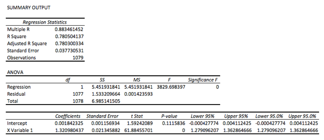
As an example of this calculation, we will examine value stocks.  Using data from the Kenneth French data library, we regress the excess returns of value stocks against the excess returns of the broad market[1].

While the analysis spits out a variety of summary statistics, the first thing most people look at are the coefficients.  The X Variable 1 here is the beta of value stocks versus the market and the Intercept is our alpha value.

The result?  According to this regression, 18 basis points (“bps”) of alpha per month.  That’s over 200 bps a year.  Hey, that’s not bad at all!

Except we’re completely ignoring the next column: standard error.  Standard error reminds us that the seemingly precise number we calculated for alpha is actually cloaked in a probability distribution.  We don’t actually know alpha – we’re trying to estimate it with data.  Despite having a significant amount of it, the data still contains quite a bit of noise and our model is by no means a perfect fit.  Therefore, our regression coefficient estimates are not singular, precise values but rather estimates that carry varying degrees of uncertainty.

In this case, the standard error for our alpha is so large (11bps per month) that we cannot conclude, at a 95% confidence level, that the true value of alpha is not actually zero.

We’re going to repeat that for emphasis: despite calculating an alpha of 18bps per month, there is enough noise in the data we used that we cannot conclude that the true alpha value is not actually zero.

This isn’t a problem if you understand it.  The problem is that nobody seems to report this uncertainty.  For example, head over to Morningstar.com and punch in any mutual fund ticker (with at least 3-years of history) and then click on the “Ratings & Risk” tab.  What you’ll find are summary statistics for beta and alpha.

What is glaringly missing is any discussion of uncertainty in these figures.  Instead, they are presented as if they are the singular true values, when in reality they may be statistically meaningless.

Without the standard error, the coefficient value is completely worthless and impossible to interpret.  Yet standard error is almost never reported.

The Takeaway: Alpha is an estimate based on statistical techniques.  Without evaluating the degree of uncertainty in that estimate, the estimate itself loses meaning.

What about epsilon?

In our simple model, we’re estimating the monthly excess returns of the investment strategy as a simple combination of a constant plus some exposure to the market’s excess return.  While hopefully accurate over the long run, we certainly don’t expect this model to be perfect each and every month.  Those monthly differences get wrapped up in the error term that trails at the end of the equation: epsilon.

In theory, epsilon is independent from month-to-month and the average value is zero.

In other words, if we hold the strategy long enough, it is diversified away over time.  Furthermore, since it is idiosyncratic risk to the strategy, we can also theoretically diversify it away by simultaneously investing in other strategies.

Theory and reality – or in this case, practice – do not always align.  While this noise term can be diversified away, the practice of reviewing manager performance on a quarterly or annual basis actually shines a very strong spotlight right on it.

In our example regression, the monthly standard deviation of error terms is 377bps.

Since we model alpha as a constant and epsilon as a zero-mean normal random variable, we can also conceptually join these two together and simply treat alpha itself as a random variable.

So in this case, we would say that while our expected alpha is 18bps (and even that is suspect, given our above discussion), it has a standard deviation of 377bps.

Which, in our opinion, re-frames the entire conversation about alpha.

Alpha is no longer a risk-free constant.  Alpha comes with its own risk.  We cannot expect to earn it each and every year.  We have to expect some random variation over time.

Furthermore, it’s crucial to compare the expected value (18bps in our example) with the standard deviation (377bps).  Through this comparison, we immediately understand that most traditional investment timeframes (e.g. 1-, 3-, 5- years) are going to be dominated by noise instead of signal. In fact, in our example, we would need a holding period of more than 15 years before we could be even 75% confident of realizing positive alpha over the investment horizon[2], despite the fact that true alpha is indeed positive.

Yet you won’t find any statistics about epsilon on almost any strategy summary reports.

The Takeaway: Epsilon, the error term, often goes unreported.  The standard deviation of this error term, however, often swamps the magnitude of the alpha estimate, and can dominate short- and even long-run performance.  Without an idea of how large the error terms can be relative to alpha, we may mistake luck, good and bad, for skill (or lack thereof).

Alpha’s Model Dependence

In 1993, Eugene Fama and Kenneth French introduced their 3-Factor model.  The model extended that traditional single factor CAPM model with two new drivers of return: the excess return generated by small-cap stocks over large-cap stocks (known as small-minus-big, or “SMB”) and the excess return generated by cheap stocks over expensive ones (known as high-minus-low, or “HML”).

Fama and French found that extending the CAPM model with SMB and HML helped more robustly explain stock returns, eliminating what in many cases had previously been identified as alpha and instead classifying it as exposure to these two new risk factors.

While these new risk factors historically generated excess risk-adjusted returns relative to the market, the idea is that they are not a truly unique source of alpha since investors can easily and cheaply access them. Therefore, a manager should not be given credit for returns coming from these sources.

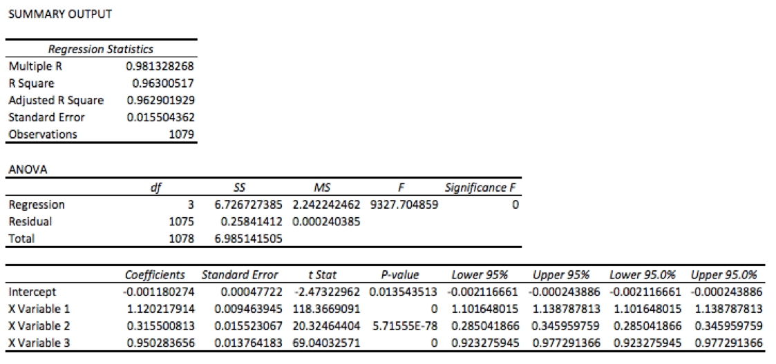
If we run the same analysis from before, but now include SMB and HML, we get a very different picture.

We find that our estimate of alpha is now negative (and statistically significantly negative, as well).  In other words, once we controlled for these risk factors, passive exposure to value stocks is no longer an alpha generating strategy.

So with one model, we have positive – though statistically insignificant – alpha; with another we have negative – and statistically significant – alpha.

Which tells us something important: our measure of alpha is highly model dependent.  The corollary here is that if the model is not adequately parameterized, latent risk factors can artificially inflate alpha.

So we may believe we’ve struck a unique vein of alpha when in reality we’ve simply allocated to an unidentified risk factor.

It is worth pointing out that they are called risk factors because investors are being compensated for bearing risk.  Alpha, theoretically, is riskless.  The dilemma here, of course, is that if we do not have the right model, we may believe certain returns are riskless when in reality they are actually quite risky.

The Takeaway: The measure of alpha is highly dependent on the risk factors used in the regression model.  Failing to adequately account for all possible risk factors can lead to an artificially inflated alpha value.

Conclusion

Alpha is not only elusive for managers to capture, but also for investors to measure.  Traditional measures and reports of alpha often fail to control for the statistical artifacts that can significantly alter the meaning of reported numbers.  Without an understanding of what risk factors were utilized in the model, the degree of certainty we have in our alpha measure, and the variance that exists in our error terms, the applicability of any alpha figure converges towards zero.

[1] As measured by the top quintile of book-to-market equities

[2] Assuming, of course, that our numerical estimates are accurate.

Copyright © Newfound Research