On Backtesting: An All-New Chapter from our Adaptive Asset Allocation Book

On Backtesting: An All-New Chapter from our Adaptive Asset Allocation Book

by Adam Butler, ReSolve Asset Management, via GestaltU

If you’ve been a regular reader of our blog, you already know that we recently published our first book Adaptive Asset Allocation: Dynamic Portfolios to Profit in Good Times – and Bad.  As of this writing, it still stands as the #1 new release in Amazon’s Business Finance category.  We’re pretty psyched about that.

In our book, we spent a great deal of time summarizing the research posted to GestaltU over the years.  We did this in order to distill the most salient points, and also to tie seemingly disparate topics together into a cohesive narrative.  Our book covers topics ranging from psychology to cognitive biases to asset valuations to retirement income planning to (of course) investment strategies.  The book was meant to stand as a single source for what ought to matter to modern investors.  As one ad for our book reads:

We hope we succeeded in doing that, but like any greatest hits album, we also included some fresh, now “tracks” in our book!  And we thought we’d share one of them with you today.  So without further ado, here’s Chapter 37, on The Usefulness and Uselessness of Backtests.

Chapter 37: The Usefulness and Uselessness of Backtests

There is a Grand Canyon-sized gap between the best and worst that backtesting has to offer. And since this book’s findings on the value of Adaptive Asset Allocation are largely based on modeled investment results, it’s only proper to include an essay on the various sources of performance decay.

The greatest fear in empirical finance is that the out of sample results for a strategy under investigation will be materially weaker than the results derived from testing. We know this from experience. When we first discovered systematic investing, our instincts were to find as many ways to measure and filter time series as could fit on an Excel worksheet. Imagine a boy who had tasted an inspired bouillabaisse for the first time, and just had to try to replicate it personally. But rather than explore the endless nuance of French cuisine, the boy just threw every conceivable French herb into the pot at once.

To wit, one of our early designs had no less than 37 inputs, including filters related to regressions, moving averages, raw momentum, technical indicators like RSI and stochastics, as well as fancier trend and mean reversion filters like TSI, DVI, DVO, and a host of other three and four letter acronyms. Each indicator was finely tuned to optimal values in order to maximize historical returns, and these values changed as we optimized against different securities. At one point we designed a system to trade the iShares Russell 2000 ETF (IWM) with a historical return above 50% and a Sharpe ratio over 4.

These are the kinds of systems that perform incredibly well in hindsight and then blow up in production, and that’s exactly what happened. We applied the IWM system to time US stocks for a few weeks with a small pool of personal money, and lost 25%.

Degrees of Freedom

The problem with complicated systems is that they require you to find the exact perfect point of optimization in many different dimensions – in our case, 37. To understand what we mean by that, imagine trying to create a tasty dish with 37 different ingredients. How could you ever find the perfect combination? A little more salt may bring out the flavor of the rosemary, but might overpower the truffle oil. What to do? Add more salt and more truffle oil? But more truffle oil may not complement the earthiness of the chanterelles.

It isn’t enough to simply find the local optimum for each input individually, any more than you can decide on the optimal amount of any ingredient in a dish without considering its impact on the other ingredients. That’s because, in most cases the signal from one input interacts with other inputs in non-linear ways. For example, if you operate with two filters in combination – say a moving average cross and an oscillator – you are no longer concerned about the optimal length of the moving average(s) or the lookback periods for the oscillator independently. Rather, you must examine the results of the oscillator during periods where the price is above the moving average, and again when the price is below the moving average. You may find that the oscillator behaves quite differently when the moving average filter is in one state than it does in another state. Further, you may discover that the effects are quite different at shorter moving average horizons than longer horizons.

To give you an idea of the scope of this challenge, consider a gross simplification where each filter has just 2 possible settings. With 37 filters we would be faced with 137 billion possible filter settings. While this permutations may not seem like a simplification, consider that many of the inputs in our 37 dimension IWM system had two or three parameters of their own (short lookback, long lookback, z score, p value, etc.), and each of those parameters was also optimized.

Never mind finding a needle in a haystack, this is like finding one particular grain of sand amongst every grain of sand on earth.

As a rule, the more degrees of freedom your model has, the greater the sample size that is required to prove statistical significance. The converse is also true: given a fixed observation horizon (sample size), a model with fewer degrees of freedom is likely to have higher statistical significance. In the investing world, if you are looking at back-tested results of two investment models with similar performance, you should generally have more confidence in the model with fewer degrees of freedom. At the very least, we can say that the results from that model would have greater statistical significance, and a higher likelihood of delivering results in production that are consistent with those observed in simulation.

Sample Size

There is another problem as well: each time you divide the system into two or more states you definitionally reduce the number of observations in each state. To illustrate, consider our 2 state example with 137 billion combinations. Recall that statistical significance depends on the number of observations, so reducing the number of observations per state of the system reduces the statistical significance. For example, take a daily rebalanced system with 20 years of testing history. If you divide a 20 year (~5000 day) period into 137 billion possible states, each state will have on average only 5000/137 billion=0.00000004 observations! Clearly 20 years of history isn’t enough to have any confidence in this system; one would need a testing period of more than 3 million years to derive statistical significance.

Degrees of freedom and sample size are two sides of the same coin. The greater the former, so too must be the latter to achieve statistical significance. Unfortunately, many models suffer from a great disconnect: insufficient sample size given the degrees of freedom. In these cases the error term dominates the outcomes and weird things happen more often than your intuition would lead you to believe. But such is the way of the world when you suffer from small sample sizes.

The problem becomes, then, how to tell a good strategy from a bad one. Most investors would seek some confidence from observing historical returns. However, investment outcomes are mostly dominated by luck over periods that most investors use for evaluation. Consider two investment teams where one – Alpha Manager – has genuine skill while the other – Beta Manager – is a closet indexer with no skill. After fees Alpha Manager expects to deliver a mean return of 10% per year with 16% volatility, while Beta Manager expects to deliver 8% with 18% volatility. Both managers are diversified equity managers, so the correlation of monthly returns is 0.95.

With some simple math (well it’s simple if you know it!), and assuming a risk free rate of 1.5%, we can determine that Alpha Manager expects to deliver about 3% per year in alpha relative to Beta Manager. This alpha is the investment measure of “raw talent.”

The question is, how long would we need to observe the performance of these managers in order to confidently (in a statistical sense) identify Alpha Manager’s skill relative to Beta Manager? Without going too far down the rabbit hole with complicated statistics, Figure 37-1 charts the probability that Alpha Manager will have delivered higher compound performance than Beta Manager at time horizons from 1 year through 20 years.

Figure 37-1. Probability Alpha Manager Outperforms Beta manager over 1-20 Years

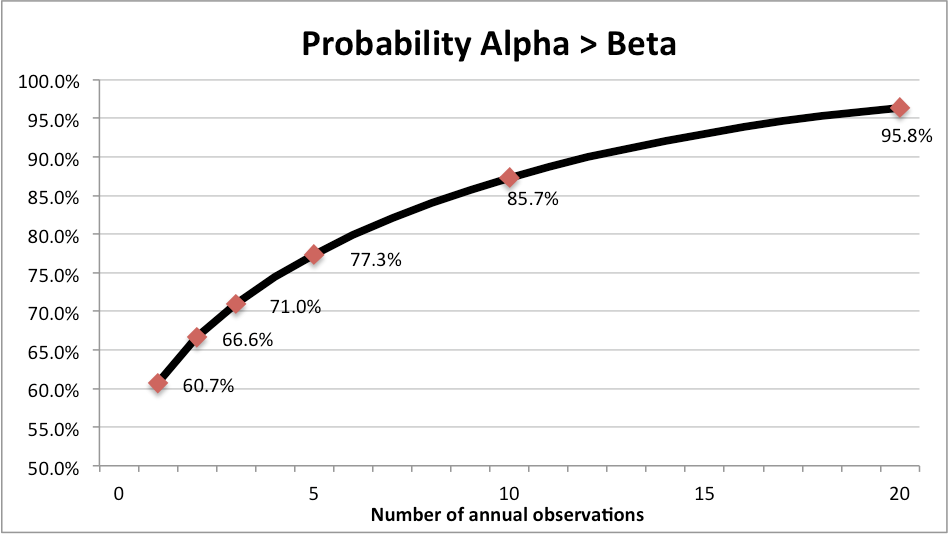You can see from the chart that there is a 61% chance that Alpha Manager will outperform Beta Manager in year 1 of our observation period. However, over any random 5-year period Beta Manager will outperform Alpha Manager about a quarter of the time, and over 10 years Beta will outperform Alpha almost 15% of the time. Only after 20 years can we finally reject the probability that Alpha Manager has no skill at the traditional level of statistical significance (5%).

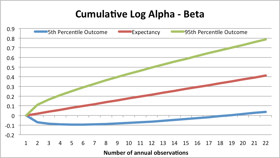
Figure 37-2 demonstrates the same concept but in a different way. The middle line represents the expected cumulative log excess returns to Alpha Manager relative to Beta Manager; note how it shows a nice steady accumulation of alpha as Alpha Manager outperforms Beta Manager each and every year. But this line is a unicorn. In reality, 90% of the time (assuming a normal distribution, which admittedly is naive) Alpha’s performance relative to Beta will fall between the top line at the high end (if Alpha Manager gets really lucky AND Beta Manager is very unlucky) and the bottom line at the low end (if Alpha Manager is really unlucky AND Beta Manger is really lucky). Note how in 5% of possible scenarios Alpha Manager is still under performing Beta Manager after 17 years of observation!

Figure 37-2. 90% range of log cumulative relative returns between Manager A and Manager B at various horizons

These results should blow your mind. They should also prompt a material overhaul of your manager selection process. But we’re not done yet, because the results above make very simplistic assumptions about the distribution of annual returns. Specifically, they assume that returns are independent and identically distributed, which they decidedly are not. In addition, certain equity factors go in and out of style, persisting very strongly for 5 to 7 years and then vanishing for similarly long periods. Dividend stocks are this cycle’s darlings, but previous cycles saw investors fall in love with emerging markets (mid-aughts), large cap growth stocks (late 1990s), large cap “nifty fifty” stocks (60s and 70s), and so on.

Basically, investment managers sometimes don’t fade with a whimper, but rather go out with a bang. So what’s an investor to do if meaningful decisions cannot be made on the basis of track records? The answer is simple: Focus on process. The most important information that is meaningful to investment allocation decisions is the process that a manager follows in order to harness one or more factors that have delivered persistent performance for many years.

The best factors have demonstrable efficacy back for many decades, and perhaps even centuries. For example, the momentum factor was recently shown to have existed for 212 years in stocks, and over 100 years for other asset classes. Now that’s something you can count on. And that’s why we spend so much time on process – because we know that in the end, that’s the only thing that an investor can truly base a decision on.

For the same reason, we are never impressed solely by the stated performance of any backtest – even our own. Rather, we are much more impressed by the ability of a model to stand up under intense statistical scrutiny: many variations of investment universes tested in multiple currencies under several regimes, along with a wide range of strong parameters with few degrees of freedom.

Often, we see advertisements of excellent medium-term results built on flimsy statistical grounds. Without understanding their process in great detail, these results are absolutely meaningless. Less commonly, we see impressive shorter-term simulations, but that are clearly based on robust, statistically-significant foundations. In those cases, we sit up and take note because thoughtful, statistically-significant, stable, results are much rarer and much more important than most investors imagine.

The investment results portrayed in marketing pieces are often nothing more than mirages. Small sample sizes, undisclosed factor exposures, and high levels of covariance between many investment strategies make it almost impossible to distinguish talent from luck over most investors’ investment horizons. In contrast, by gaining a deep understanding of the process that gives a manager an edge, with credible statistical substantiation, an investor can have measurable confidence in the prospects of a strategy.

Of course, once a strategy is widely recognized as being successful, it is likely to start attracting more capital. As a result, a meaningful portion of observed out-of-sample performance decay is the result of arbitrage; that is, others discovering and concurrently exploiting the same anomaly.

Multiple Discovery

One of the more interesting marvels observed over the centuries in science is “multiple discovery.” This phenomenon, so named by noted sociologist Robert K. Merton in 1963 (not to be confused with Robert C. Merton, who won the Nobel Prize in Economics for co-publishing the Black-Scholes-Merton option pricing model), occurs when two or more researchers stumble on the same discovery at nearly the same time, but without any prior collaboration or contact. Historically, these discoveries happened almost concurrently in completely different parts of the world, despite little shared scientific literature, and significant language barriers.

For example Newton, Fermat and Leibniz each independently discovered calculus within about 20 years of each other in the late 17th century. Within 15 years of each other in the 16th century, Ferro and Tartaglia independently discovered a method for solving cubic equations. Robert Boyle and Edme Mariotte independently discovered the fundamental basis for the Ideal Gas Law within 14 years of each other in the late 17th century. Carl Wilhelm Scheele discovered Oxygen in Uppsala, Sweden in 1773, just 1 year before Joseph Priestley discovered it in southern England. Both Laplace and Michell proposed the concept of “black holes” just prior to the turn of the 18th century.

The 19th and 20th centuries also saw a wide variety of multiple discoveries, from electromagnetic induction (Faraday and Henry), the telegraph (Wheatstone and Morse in the same year!), evolution (Darwin and Wallace), and the periodic table of the elements (Mendeleev and Meyer). Alan Turing and Emil Post both proposed the “universal computing machine” in 1936. Jonas Salk, Albert Sabin and Hilary Koprowski independently formulated a vaccine for polio between 1950 and 1963. Elisha Gray and Alexander Graham Bell filed independent patents for the telephone on the same day in 1876!

Though not at all a complete list, Wikipedia has catalogued well over 100 instances of multiple discovery in just the past two centuries. If the frequency of multiple discovery is related to both the speed of communication and the number of linked nodes in a research community (a hypothesis for which we have no proof, but that is logically appealing), then the concept of multiple discovery has important implications for current investors in the age of the Internet.

For us, there is a clear analog in quantitative finance: researchers operating independently, but sourcing ideas from a common reservoir will almost certainly stumble on similar discoveries at approximately the same time. This dynamic will almost certainly lead to some performance decay once these strategies are put to work out of sample, and with real money, as all of these investors will be attempting to draw from the same well of alpha. Indeed, in a recent paper Jing-Zhi Huang and Zhijian (James) Huang demonstrate that published anomalies exhibit meaningful performance decay after publication, though the best anomalies, such as value and momentum, do preserve much of their pre-publishing luster out of sample.

Structural Impediments to Asset Class Arbitrage

It’s important to note that the anomalies explored by Huang and Huang relate specifically to equity selection. We believe active approaches to global asset allocation have several advantages, in terms of sustainability, over strategies aimed at selecting securities within a specific asset class. As a result, we expect them to be less vulnerable to decay.

For example, most investors have a strong home bias and are not open to approaches that stray too far from stocks and bonds of their country of residence. Strategies that propose to be agnostic to home bias, and spend substantial periods invested in unfamiliar assets are unlikely to gain mass adoption.

More importantly, major asset classes represent enormous pockets of capital, on the order of hundreds of billions, or even trillions, of dollars. Markets this deep require equally deep sources of capital to arbitrage. Yet the current large sources of capital in global markets – pensions, endowments, and other institutions – are constrained in their ability to take advantage of the opportunity in this space in three important ways:

1. Many of these institutions are structured along asset class lines, with resources dedicated to each asset class silo individually. Dynamic asset allocation might see one silo receive very little capital allocation for many months or years; it is difficult to lay off employees and recall them when their asset class is back in favor.
2. Where asset allocation is implemented through outside managers, dynamically shifting across asset classes would require frequent redemptions and reallocations, which may not align with longer-term security selection strategies. Many more successful strategies would not accept such active rotation in and out of their funds, and may choose to limit access to institutions who frequently reallocate.
3. Many, if not most, institutions are managed by large boards with diverse experience and skill-sets. These boards meet infrequently, but are responsible for approving large shifts in strategy. It would represent a large departure from convention for a board to approve a meaningful shift into such a novel approach, about which most if not all of the board members have little to no experience.

For these and other reasons, we feel global multi-asset active allocation strategies have many strong years ahead of them, in contrast to many other strategies, which may live and die very quickly because they do not possess the above characteristics.

On the Robustness of Adaptive Asset Allocation

There is a common misconception – that even our younger selves once held – that the primary goal of investment modeling is to maximize backtest results. But the catastrophic failure of our 37-dimensional system, along with countless smaller but no less important lessons over the past six years, have helped us to see the light. No, as we’ve now mostly internalized, the primary goal of investment modeling is to develop systems where the distribution of in-sample returns maximally reflects the distribution of real-world returns. This is the definition of robustness.

As we’ve discussed, there are ways to maximize robustness: minimize degrees of freedom, maximize sample size and invest in ways that structurally limit arbitrage. Our formulation of Adaptive Asset Allocation has all of these characteristics. By using a global asset class-based approach with minimal degrees of freedom tested over multiple economic regimes, we maximize the odds that future outcomes will resemble the past.

We don’t know what’s going to happen tomorrow. Nobody does. But in the end, we are confident that the Adaptive Asset Allocation approach will continue to deliver in-line with our expectations.

And in the world of investing, what more could you ask for?

Copyright © GestaltU